

Deduplication & Compression Ratio Calculator
This Deduplication & Compression Ratio Calculator shows how much physical storage your data occupies after deduplication and compression are applied. Enter your Logical Data Size and unit, then set your Deduplication Ratio and Compression Ratio — or pick a workload preset — and click Calculate Savings to see physical storage required, total space saved, and the combined data reduction ratio: the multiplier that tells you how far your physical hardware actually goes. Also see: Data Transfer Time Calculator.
Effective Capacity and Space Savings After Dedup and Compression
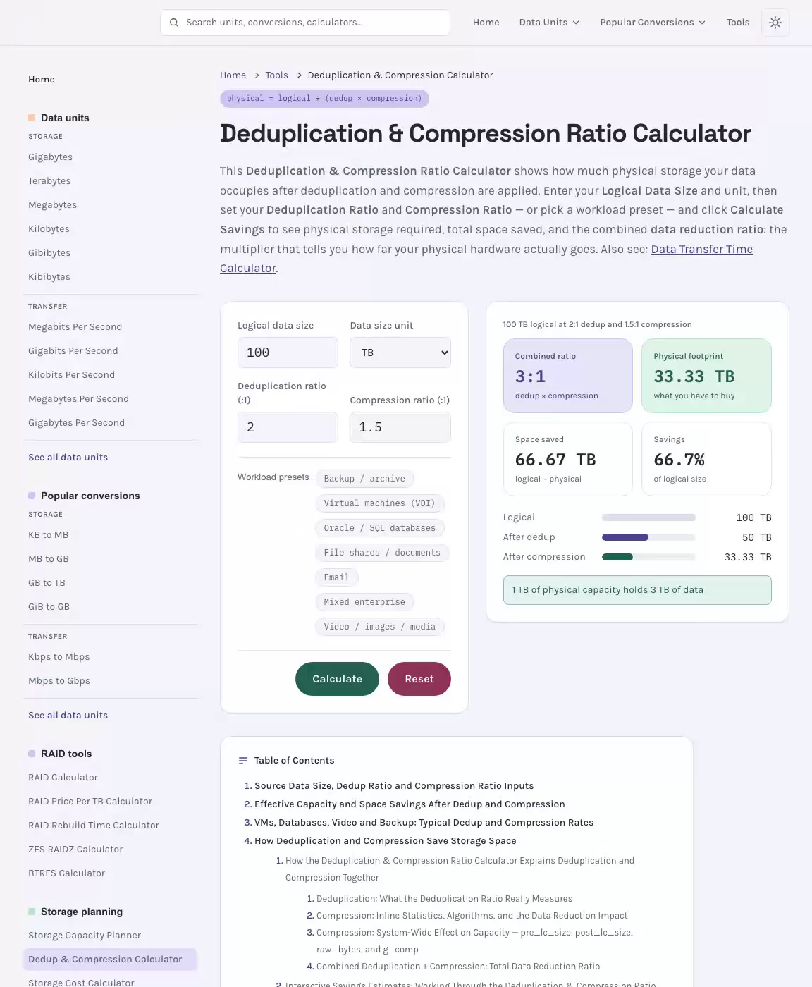
100 TB logical at 2:1 dedup and 1.5:1 compression
Combined ratio
dedup × compression
Physical footprint
what you have to buy
Space saved
logical − physical
Savings
of logical size
- Logical
- After dedup
- After compression
1 TB of physical capacity holds 3 TB of data
VMs, Databases, Video and Backup: Typical Dedup and Compression Rates
| Workload Type | Dedup Ratio | Compression Ratio | Combined (typical) | Notes |
|---|---|---|---|---|
| Backup / Archive | 10–20:1 | 1.5–2:1 | 15–40:1 | Best case; repeated versions of same files |
| Virtual Machines (VDI) | 3–5:1 | 1.5–2:1 | 5–10:1 | Shared OS images across many VMs |
| Oracle / SQL Databases | 2–5:1 | 2–4:1 | 4–10:1 | Highly repetitive row/index structures |
| File Shares / Documents | 2–4:1 | 1.5–3:1 | 3–8:1 | Office files and text compress well |
| 2–3:1 | 1.5–2:1 | 3–5:1 | Repeated attachments benefit from dedup | |
| Mixed Enterprise | 2–3:1 | 1.5–2:1 | 3–5:1 | HPE/NetApp vendor typical claim |
| Video / Images / Media | 1:1 | 1:1 | 1:1 | Pre-compressed; no reduction possible |
How Deduplication and Compression Save Storage Space
When you're trying to plan capacity for an enterprise recovery environment, the gap between what vendors advertise and what you actually experience on disk can be enormous — and expensive. Use this deduplication & compression ratio calculator above to get a precise picture of your true physical footprint by separating deduplication savings from compression savings and combining them into a real, usable data reduction ratio (DRR). Whether you're sizing a new purpose-built appliance deployment, validating a vSAN environment before entering full data migration maintenance mode, or simply trying to understand why your recovery appliance reports a 46x ratio, this tool cuts through the marketing math and grounds your capacity planning in real numbers. Applying compression deduplication techniques correctly requires understanding both layers — and the post-compression physical footprint that results from combining them — to achieve meaningful storage optimization and cyber resilience in production environments.
See the Dedup & Compression Calculator in Action
How the Deduplication & Compression Ratio Calculator Explains Deduplication and Compression Together
Deduplication: What the Deduplication Ratio Really Measures
Deduplication is a process that prevents the same data from being stored again — ensuring no data stored again wastes physical capacity. When an incoming data segment arrives at a deduplication file system, the system checks whether an identical unique segment already exists in the deduplication scope. If it does, only a reference pointer is stored rather than a second physical copy, which eliminates redundancy at the block or segment level. This is fundamentally different from compression, which encodes a single stream of data more efficiently — deduplication prevents redundant blocks from occupying physical space in the first place. Related: Storage Throughput Converter.
The deduplication ratio (sometimes called the dedupe ratio or dedup ratio) is expressed as:
This means the ratio is a comparison between the logical data footprint — all the data your protection software would have written without deduplication — and the physical space consumed after redundant segments have been eliminated. Understanding this distinction is critical for capacity sizing, because many vendors report deduplication ratios using the inflated total managed figure in the numerator, which makes ratios appear far more impressive than everyday operational reality would suggest.
Inline deduplication processes incoming data segments in real time before they are written to disk. Post-process deduplication, by contrast, writes data first and deduplicates later in a background pass. Most modern purpose-built appliance platforms — including Data Domain systems — use inline deduplication so that only unique blocks ever touch the disk, maximising both efficiency and throughput. The deduplication procedure examines each incoming segment against an index of previously stored unique data segments and routes it accordingly.
In virtual environments using virtualization infrastructure, native deduplication effectiveness is especially high because virtual machines often share identical OS images, application binaries, and base disk blocks. Across a vSAN environment with deduplication enabled, a single independent deduplication scope can eliminate enormous volumes of repetitive content across multiple VMs sharing the same golden image. For protected workloads, the deduplication impact depends heavily on how much redundant content arrives — which is directly tied to the protection strategy (full vs. incremental) and the daily modification rate.
Compression: Inline Statistics, Algorithms, and the Data Reduction Impact
Compression reduces the logical size of data by encoding it more efficiently, without (in the case of lossless compression) discarding any information. On Data Domain and similar DDOS platforms, compression operates at multiple layers, each reported separately in the compression statistics output of filesys show compression. Understanding these layers is essential to correctly interpreting the numbers your system reports.
The three primary compression algorithms available on Data Domain systems are lz, gzfast, and gz — listed here from fastest/lowest ratio to slowest/highest ratio. Your choice of algorithm represents a tradeoff between CPU overhead and space reduction. The table below summarises typical effective compression ratio ranges by algorithm:
| Compression Algorithm | CPU Impact | Typical Compression Ratio Range | Best Use Case |
|---|---|---|---|
| lz | Low | 1.2:1 – 1.8:1 | High-throughput, latency-sensitive workloads |
| gzfast | Medium | 1.8:1 – 2.5:1 | Balanced throughput and compression effectiveness |
| gz | High | 2.5:1 – 4.0:1 | Archiving and long-retention protected datasets |
The filesys show compression command outputs inline compression statistics across four key columns: Pre-Comp (data written before compression, in GiB), Post-Comp (space used after encoding), Global-Comp Factor, and Local-Comp Factor, which together produce the Total-Comp Factor (also called total compression factor). A representative output looks like this:
Mtree: /data/col1/backup-mtree
# filesys show compression

From: 2023-12-31 03:00 To: 2024-01-07 03:00
Active Tier:
            Pre-Comp   Post-Comp   Global-Comp   Local-Comp   Total-Comp
               (GiB)       (GiB)        Factor       Factor       Factor
                                                             (Reduction)
  Daily:
  2024-01-01   1024.0      410.2          1.45         1.71         2.50x
  2024-01-02   1018.5      402.9          1.47         1.72         2.52x
  ...
  Weekly:      7143.5     2876.4          1.46         1.71         2.48x
  Last 24 Hrs:  1021.2      409.1          1.45         1.71         2.49x
  Last 7 Days: 7143.5     2876.4          1.46         1.71         2.48x
  Last 33 Days:30012.0    12040.8          1.45         1.70         2.49x
Cumulative:   45000.0    18032.4          1.45         1.72         2.50x
In this output, the pre-comp column reflects data written before compression — your logical bytes before any encoding. The post-comp column shows the space used after encoding. The local compression ratio (local-comp factor, also called FSC — File System Compression) represents the inline encoding applied at write time within the active namespace. The global compression factor (g_comp, also called MSC — Meta-data System Compression) reflects additional gain achieved by the log-structured file system through garbage collection and data reorganisation — this is where the deduplication file system's log-structured nature produces extra savings beyond what inline encoding achieves.
The distinction between static encoding ratio and dynamic effective compression ratio is important for capacity planning. The static figure is a fixed, algorithm-specific value describing a single data stream. The dynamic effective compression ratio — also called the system effective compression ratio or overall encoding ratio — reflects the actual ratio observed across your entire active layer over time, accounting for content types, entropy levels, pre-compressed file formats, and pre-encrypted content that resists further compression. The dynamic figure is always the one reported in cumulative compression statistics and is the one you should use for capacity sizing.
Compression: System-Wide Effect on Capacity — pre_lc_size, post_lc_size, raw_bytes, and g_comp
To correctly calculate the effective compression ratio at the file system level, you need to understand how three internal metrics relate to each other. These values appear in Mtree-level compression output and in low-level system diagnostics:
- raw_bytes: The original bytes written by the protection application — the logical size of content before any deduplication or compression processing. This represents the pre-compression volume at the front-end data size level.
- pre_lc_size: The size of content after deduplication but before local compression is applied. This is the pre-comp size you see reported in compression statistics — the volume after de-dupe but before file compression encoding.
- post_lc_size: The size after local compression — the post-comp size, representing content written to the primary tier after inline encoding has been applied.
From these three values, you can derive both the local encoding factor and the dedupe impact independently:
The g_comp factor accounts for savings from the log-structured file system's space reclamation and garbage collection cleaning passes, as well as savings from features like fast copy and virtual synthetics. Fast copy operations create new recovery images by referencing existing unique data segments rather than rewriting content — this produces large apparent logical capacity figures without consuming additional physical space, which can make compression statistics appear more favourable than a simple pre/post measurement would suggest. Virtual synthetics similarly assemble complete recovery images from existing incremental snapshot segments, producing high logical bytes written with minimal physical space actually used.
The filesys show space command gives you the top-level view of capacity used vs. logical capacity used for the entire system, while the mtree show compression command provides per-Mtree reporting, and mtree list enumerates all active Mtrees in the deduplication scope:
# filesys show space

Resource           Size GiB   Used GiB  Avail GiB  Use%
-------------------  -------  ---------  ---------  ----
/data: pre-comp         65000      45000          -    -
/data: post-comp        65000      18032      46968   28%
/ddvar                    100         18         82   18%

Data Domain File System status: Enabled, Running

# mtree show compression /data/col1/backup-mtree

                Pre-Comp   Post-Comp   Global-Comp   Local-Comp   Total-Comp
                   (GiB)       (GiB)        Factor       Factor       Factor
Cumulative:    45000.0     18032.4          1.45         1.72         2.50x
For cloud tier configurations on Data Domain, the reported compression statistics include an additional layer reflecting data movement to object repositories. Cloud tier migration produces a separate reported ratio because the cloud layer stores content in a different format optimised for object bandwidth rather than flash storage read/write performance. The globally compressed and locally compressed figures for the cloud tier are reported separately from the primary tier, so your system-level statistics must account for both tiers to get an accurate total-comp factor across your entire data footprint. Non-cloud Data Domain configurations report a unified primary tier figure without this split.
Combined Deduplication + Compression: Total Data Reduction Ratio
The combined reduction ratio — the number most commonly cited in vendor marketing and the value this calculator computes — is the product of your deduplication ratio and your effective compression ratio applied sequentially to the same logical collection:
Total Data Reduction Ratio = Deduplication Ratio × Effective Compression RatioAlternatively, it can be expressed directly as:
This is the figure reported as the system effective compression ratio in DDOS terminology — the ratio of all logical bytes ever written to the system against the used physical space on disk after all deduplication, local compression, and global compression have been applied. It is a cumulative statistic, meaning it reflects the entire history of content written to the system, not just the last 24 hours or last 7 days. The time-windowed and last 33 days views give you a trending perspective that is useful for analysis but should not be confused with the system-wide cumulative figure used for capacity planning and infrastructure reporting.
Features that artificially inflate this ratio include fast copy operations, virtual synthetics, and snapshots — all of which add logical bytes to the managed-data numerator without writing new unique segments to disk. Overwrites and deletes, conversely, may reduce the logical volume but do not immediately reclaim physical space; that reclamation happens during garbage collection cleaning cycles, which are managed by the log-structured file system's space reclamation process. This time lag between logical deletes and physical space reclamation means your reported used physical space may temporarily appear higher than expected after large-scale data management operations, including retention lock expiry and archiving workflows.
Interactive Savings Estimates: Working Through the Deduplication & Compression Ratio Calculator with Real Data Scenarios
Calculating Inflated Capacity for Deduplication — the Core Sizing Problem
One of the most practically important applications of this calculator is determining how much physical capacity a vSAN environment actually needs before you initiate a full data migration maintenance mode operation. When deduplication enabled status is confirmed on a vSAN setup, inflight content transferred between volume groups during maintenance mode is not re-deduplicated — it travels as its fully inflated, pre-dedupe logical volume. This means the capacity disks on the receiving groups must have enough raw capacity to absorb the inflation amount. See also: NVMe Queue Depth Calculator.
For releases older than 6.7 U3, there is no automated pre-check in the vSphere web client, so you must manually calculate the inflation amount before entering the decom state. The process uses three values from the DISK_STATUS structure reported by cmmds-tool find:
- capacityUsed: the actual physical space consumed on the capacity disk (bytes)
- logicalCapacityUsed: the logical capacity used — what the content would occupy without deduplication (bytes)
- physDiskCapacityUsed: the total physical disk capacity used including metadata overhead
The dedupe ratio calculation at the disk level is:
And the inflated capacity (the raw capacity that will be generated when deduplication is temporarily bypassed) is simply the logicalCapacityUsed value converted from bytes to GiB by dividing three times by 1024. This is the 1024 conversion used to produce the GiB value from the raw byte count reported by the query tool. The result gives you the GiB raw figure representing how much physical space each capacity tier disk would consume if it had to store all content without dedupe/compression active — your inflation amount and your capacity check baseline.
With the release of vSAN 6.7 U3, VMware introduced an automated space check in the web client that runs this capacity check automatically as a pre-check before the server maintenance mode outcome is committed. For all environments running 6.7 U3 or later, the system will warn you if there is not enough space to safely complete the full data migration without the decom state exhausting disk capacity.
Worked Examples: Real-World Deduplication & Compression Ratio Scenarios Across Protected Content Types
The following three worked examples ground the abstract ratio math in real TB-scale values that reflect actual enterprise workloads. Each example demonstrates a different point on the deduplication effectiveness spectrum.
Example 1 — Basic Dedupe Scenario (One Week, Full + Incremental Backup):
A company protects 100TB of assorted data. The protection software performs software compression and deduplication. The initial full scheduled full backup with a 2:1 encoding factor reduces 100TB to 50TB. Subsequent daily incremental snapshots capture a 1% modification rate — that is 1TB of raw changes per day. Over 5 weekdays, that is 5TB of raw daily changes, compressed 2:1 to 2.5TB. A total of 52.5TB of content physically retained on disk after one week.
Now calculate the dedupe impact using total managed volume as the logical numerator:
- Day 0 baseline: 100TB logical
- Days 1–5 at 1TB daily modification rate: 5TB additional logical
- Total logical data under management (week 1): 105TB
105TB/52.5TB = 2x — a result that is functionally just your encoding rate, because with a single full backup plus incremental snapshots, you haven't yet generated significant redundant segments sent to the target appliance.
Example 2 — Combined Dedupe + Compression Scenario (Full Daily Backups, One Week):
Now consider the same 100TB collection, but the protection software is configured to run a complete recovery copy every day instead of incrementals. Without deduplication or compression, the content accumulates as follows:
- Day 0 (baseline): 100TB
- Day 1 (baseline + changes): 101TB
- Day 2: 102TB
- Day 3: 103TB
- Day 4: 104TB
- Day 5: 105TB
This 615TB total represents the full managed logical volume. The physically retained content remains 52.5TB (the deduplicated and compressed footprint), because subsequent full copies are almost entirely composed of redundant segments already retained during the baseline pass. Deduplication prevents the same data from being stored again, so only net-new unique blocks consume additional physical space.
615/52.5 = 11.714x — this is the combined compression deduplication ratio for one week of daily full copies. The ratio has grown dramatically from 2x simply because more redundant protected content is being represented in the logical managed volume numerator.
Example 3 — High-Ratio Enterprise Scenario (30-Day Period):
Extending the same 100TB collection with a 1% daily modification rate across a full monthly window with scheduled full backups each day:
- 30 complete recovery copies × 100TB base = 3,000TB logical
- 30 days × 1TB daily modification = 30TB additional logical content
- Total logical data under management: 3,030TB
With encoding and deduplication operating throughout, the physically retained volume grows modestly — primarily by the daily unique blocks after encoding — reaching approximately 65TB of content physically retained on the appliance:
3,030TB/65TB (content physically retained) = 46.62x — this is the kind of figure that appears in purpose-built appliance vendor datasheets. It is real, but it is critically important to understand that it reflects a specific protection strategy (daily full copies), a specific daily modification rate (1%), a specific retention window (30 days), and a specific collection composition. Change any of these variables — switch to incremental snapshots, reduce the retention to 7 days, or protect a collection with a higher daily modification rate or pre-encrypted content that resists compression — and the ratio changes significantly.
In summary:
- 100TB collection, 1% modification rate, 1 week, full backup + daily incremental backups: 52.5TB retained, 2x DRR
- 100TB collection, 1% modification rate, 1 week, daily full copies: 52.5TB retained, 11.7x DRR
- 100TB collection, 1% modification rate, 30-day period, scheduled full backups daily: ~65TB retained, 46.62x DRR
That is how purpose-built appliance deduplication ratios really work — they are a representation of what the logical data footprint would have been without deduplication, divided by what actually sits on disk. They are a math exercise built on assumptions about protection strategy, retention, and modification rate. Front-end data size, daily modification rate, and retention period are the three biggest variables that determine your expected footprint and the resulting optimization ratio you can realistically expect in production.
File Compression Fundamentals: Lossless, Lossy, and the Impact on Your Data Footprint
Beyond enterprise recovery environments, file compression methods fall into two fundamental categories that affect content volume, file quality, and reversibility. Understanding the distinction matters for capacity sizing, data transfer planning, and archiving decisions across multiple file formats.
Lossless compression retains all original information and can be completely reversed. The compressed file can be fully restored to its original state with no omission. Reversible encoding is used by formats including ZIP (rar is another common lossless method), and for images the PNG format applies lossless techniques. For text files, lossless encoding typically yields high reduction rates because text contains significant repetitive content that can be efficiently encoded. Binary prefixes apply equally to both compressed and uncompressed measurements — 1 GiB = 1024 MiB = 1024 × 1024 × 1024 bytes, so one megabyte of text may compress to a fraction of its original size while remaining fully reversible. Reversible encoding is the standard for protected datasets and database archives where data integrity is non-negotiable.
Lossy compression, by contrast, permanently discards information deemed least perceptible to the end user — making it irreversible. The JPG format applies lossy encoding to images; strong JPG settings visibly degrade image quality, demonstrating the direct tradeoff between compressed size and file quality. The MP3 format applies lossy audio encoding by discarding frequencies beyond human hearing thresholds, while MP4 applies lossy encoding to video streams. Unlike lossless methods, lossy encoding cannot be undone — if the original file is lost, the compressed format is the only remaining version. For scenarios where information retained is paramount, such as database archives, incremental snapshot chains, and compliance archiving, lossy encoding is never appropriate. Image, audio, and video encoding workflows each have their own compression limit beyond which quality loss becomes unacceptable to end users.
When you use this compression ratio calculator to calculate data compression for general file management, you enter two of three values — the uncompressed size (size before compression), the compressed size (size after encoding), and the encoding factor — and the tool derives the third. Space savings are expressed both as a ratio and as a percent savings figure, letting you immediately see the reduction % your chosen method delivers across different content categories and encoding approaches.
For enterprise infrastructure contexts, pre-compressed files (already encoded with zip or media encoding) and pre-encrypted content present a challenge for further encoding — their entropy is too high for additional passes to reduce the volume meaningfully. Sparse files similarly may report a large logical size but contain mostly zeroes, which encode extremely well with lossless methods. Small file overhead and small block size effects mean that file metadata and inode structures can add meaningful overhead relative to the actual data payload for workloads composed of many tiny digital files, making the effective encoding factor lower than the algorithm's theoretical maximum. Compression heuristics on modern systems detect pre-compressed and pre-encrypted content and skip unnecessary passes, preserving throughput and CPU resources for data that will actually benefit from encoding.
Appendix: Manual Calculation Methods, CLI Commands, and Scripting Deduplication Ratio Live
For infrastructure administration teams operating Data Domain or vSAN environments, the following CLI reference covers the key commands used to retrieve raw compression statistics and perform manual dedupe ratio calculations at the disk level and system level.
Step 1: Confirm deduplication enabled status and capture the vSAN UUID
# Run esxcli vsan storage get to determine if Deduplication/Compression is enabled.
# Note the VSAN UUID for the capacity disk.
esxcli vsan storage get

# Example relevant output:
naa.500003972c8884e9:
  Is SSD: true
  VSAN UUID: 5221c646-88b6-5622-f995-0xxxxxxxxxxb
  VSAN Disk Group UUID: 524f4373-2059-edb9-4023-9xxxxxxxxxxe
  On-disk format version: 3
  Deduplication: true
  Compression: true
  Checksum OK: true
  Is Capacity Tier: true
Step 2: Capture capacityUsed and logicalCapacityUsed from disk_status via cmmds-tool find
cmmds-tool find -f json -t DISK_STATUS -u 5221c646-88b6-5622-f995-0xxxxxxxxxxb

# Relevant fields in JSON format output:
{
  "content": "{
    \"capacityUsed\": 848886642881,
    \"logicalCapacityUsed\": 1274401521664,
    \"physDiskCapacityUsed\": 7717151298919,
    \"writeConsolidationRatio\": 10,
    \"numDataComponents\": 32
  }"
}
Step 3: Perform the dedupe ratio calculation and determine the inflation amount
# Disk-level dedupe ratio:
# logicalCapacityUsed / capacityUsed
1274401521664 / 848886642881 = 1.5x dedupe ratio

# Cap after inflation (GiB raw -- what this disk will need to hold without dedupe):
# logicalCapacityUsed divide by 1024 three times to get GiB value
1274401521664 / 1024 / 1024 / 1024 = 1186.88 GiB raw

# This is the approx GiB of raw capacity this volume group will need
# to survive full data migration without running out of space.
Scripting the calculation live — to run this automatically across all capacity disks on a vSAN node before entering decom state:
esxcli vsan storage list | grep "VSAN UUID" | awk '{print $3}' | while read i; do
  totalUsed=$(cmmds-tool find -f json -t DISK_STATUS -u $i \
    | grep -o '"logicalCapacityUsed": [0-9]*' \
    | awk '{print $2 / 1024 / 1024 / 1024}');
  echo "$i: Approx. $totalUsed GiB without dedupe/compression";
done

# Example output:
# 520e35f5-6cfd-de13-eed5-9xxxxxxxxxxf: Approx. 0 GiB without dedupe/compression
# 5280832b-f606-89c7-e481-0xxxxxxxxxx1: Approx. 72.7656 GiB without dedupe/compression
# 52b70846-56cc-d63f-a3bc-1xxxxxxxxxx3: Approx. 6.48828 GiB without dedupe/compression
Repeat this UUID iteration for each disk in the vSAN environment to determine whether there is enough space available across the entire system to safely complete entering decom without the capacity inflation amount exceeding available disk space. This scripting approach works on any node running vSAN with deduplication enabled, regardless of the on-disk format version, and gives your infrastructure team a live calculation of the true capacity check figure before committing to full data migration maintenance mode.
For Data Domain environments, the equivalent Mtree-level compression breakdown for a specific protected Mtree path is retrieved with:
# Mtree-level compression breakdown
mtree show compression /data/col1/your-mtree-name

# System-level (filesys show compression) -- cumulative and delta compression statistics:
filesys show compression

# For time-windowed view (daily option):
filesys show compression daily-detailed
These commands give you the pre_lc_size, post_lc_size, and raw_bytes relationships you need to manually derive the inline compression statistics for any Mtree or for the full deduplication scope. The periodic and weekly figures help you trend encoding effectiveness over time, while the cumulative statistics represent your system's overall ratio for capacity planning and utilisation reporting. Combine the system-level output from filesys show compression with the capacity utilisation from filesys show space to get a complete picture of your optimization story — from the logical data footprint at the protection software level all the way to the physical space consumed on your appliance disks.
Most companies protect multiple content categories across their data protection environment — database archives with low encoding rates, virtual machine images with high deduplication effectiveness, file server snapshots with strong lossless encoding, and media files that resist further compression. Each collection produces a different expected footprint and a different encoding effect. The front-end data size, daily modification rate, and retention period are the three variables with the greatest leverage on your overall combined ratio — and understanding exactly how each one feeds into the numerator of your deduplication ratio is what separates a realistic capacity sizing exercise from a marketing-driven math exercise built on inflated managed-data assumptions.
Inline vs Post-Process Dedup, Fixed vs Variable Block and Lossless Compression
Deduplication: Identifies and eliminates identical data blocks across the dataset. A 3:1 ratio means 3TB of logical data is stored in 1TB of physical space by referencing duplicate blocks rather than storing them multiple times.
Compression: Reduces the size of unique data blocks using encoding algorithms (LZ4, ZLIB, etc.). A 1.5:1 ratio means 1.5TB of data is compressed to 1TB on disk.
Combined Ratio: The product of both ratios. A 2:1 dedup and 1.5:1 compression gives a 3:1 combined ratio — meaning 3TB of data occupies only 1TB of physical storage.
Vendor Claims vs Reality: Vendors often advertise best-case ratios. Use conservative estimates (mixed enterprise: 2–3:1 combined) for capacity planning unless your workload is known to be dedup-friendly.