

IOPS Calculator
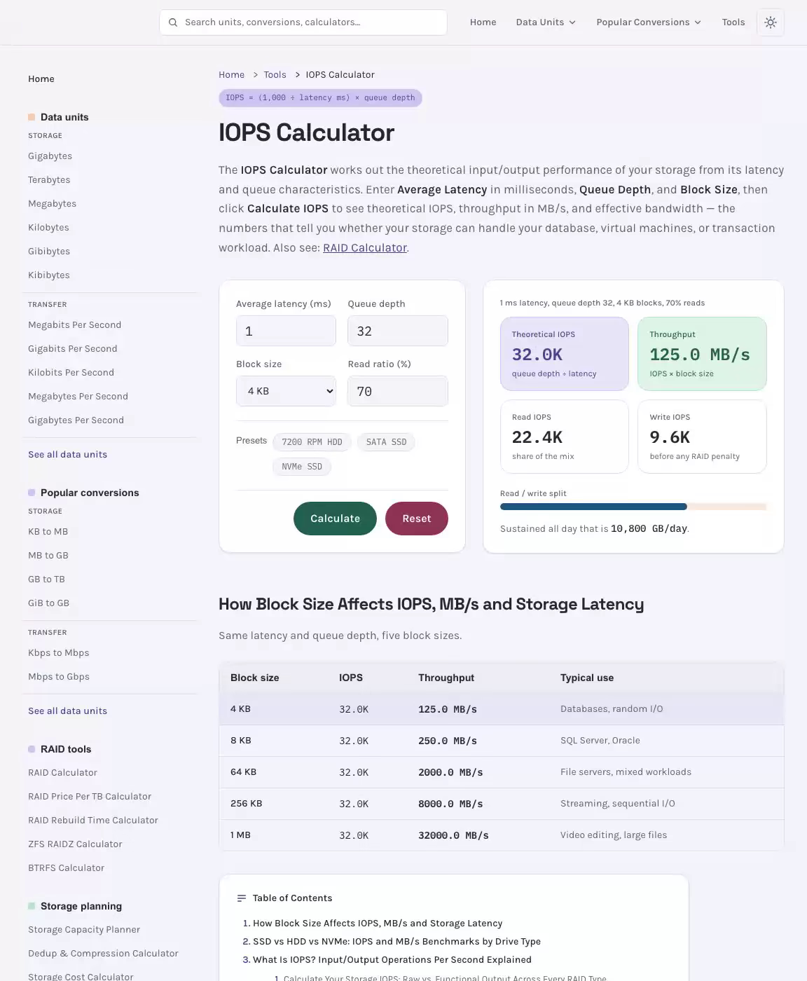
The IOPS Calculator works out the theoretical input/output performance of your storage from its latency and queue characteristics. Enter Average Latency in milliseconds, Queue Depth, and Block Size, then click Calculate IOPS to see theoretical IOPS, throughput in MB/s, and effective bandwidth — the numbers that tell you whether your storage can handle your database, virtual machines, or transaction workload. Also see: RAID Calculator.
Results
1 ms latency, queue depth 32, 4 KB blocks, 70% reads
Theoretical IOPS
queue depth ÷ latency
Throughput
IOPS × block size
Read IOPS
share of the mix
Write IOPS
before any RAID penalty
Read / write split
Sustained all day that is .
How Block Size Affects IOPS, MB/s and Storage Latency
Same latency and queue depth, five block sizes.
| Block size | IOPS | Throughput | Typical use |
|---|---|---|---|
| 4 KB | 32.0K | 125.0 MB/s | Databases, random I/O |
| 8 KB | 32.0K | 250.0 MB/s | SQL Server, Oracle |
| 64 KB | 32.0K | 2000.0 MB/s | File servers, mixed workloads |
| 256 KB | 32.0K | 8000.0 MB/s | Streaming, sequential I/O |
| 1 MB | 32.0K | 32000.0 MB/s | Video editing, large files |
SSD vs HDD vs NVMe: IOPS and MB/s Benchmarks by Drive Type
| Storage Type | Typical Latency | 4K Random IOPS | Sequential MB/s |
|---|---|---|---|
| 7200 RPM HDD | 8-12 ms | 75-150 | 100-200 |
| 10K RPM HDD | 5-8 ms | 150-250 | 150-250 |
| 15K RPM HDD | 3-5 ms | 200-350 | 200-300 |
| SATA SSD | 0.1-0.5 ms | 50K-100K | 400-550 |
| NVMe SSD | 0.02-0.1 ms | 100K-1M+ | 3,000-7,000 |
| Intel Optane | 0.01 ms | 500K-2M+ | 2,500-3,000 |
What Is IOPS? Input/Output Operations Per Second Explained
Planning a new storage infrastructure or sizing a redundant array for your next database or virtualization project? The iops calculator gives you the effective throughput, aggregate drive output, and data transfer MB/s your configuration will actually deliver — not just the theoretical peak. Whether you are choosing between a budget 7.2K SATA spinning drive array and a high-density flash cluster, understanding how your array configuration drains disk performance through its overhead is what separates a well-designed server from an expensive bottleneck. This drive estimator and gb/day converter bridges the gap between spec sheets and real-world throughput so you can make confident, data-backed decisions before you buy a single drive.
See the IOPS Calculator in Action
Calculate Your Storage IOPS: Raw vs. Functional Output Across Every RAID Type
Every storage calculation starts with two distinct numbers: the aggregate drive output your physical drives can theoretically deliver, and the effective output your application task will see after accounting for array overhead, read/write mix, and the real-world mechanics of drive I/O. This iops calculator acts as an estimator and converter for both figures simultaneously, letting you model everything from a cost-sensitive spinning-drive array to an enterprise flash configuration tuned for virtual environments or high-frequency databases. Use it to calculate storage requirements before committing to hardware, and to understand input/output operations per second in the context of your chosen redundancy scheme. Related: RAID Rebuild Time Calculator.
Functional vs. Raw IOPS: Understanding Your Actual IOPS After RAID Penalty
Raw IOPS is the sum of every drive's individual IOPS contribution before any array logic is applied. If you install ten 7.2K SATA spinning drives rated at 75–100 IOPS each, your aggregate total sits between 750 and 1,000 IOPS. That sounds straightforward — but redundant arrays introduce additional write operations behind the scenes, and those extra operations reduce the number of application-visible write commands the array can service per second. The result is effective IOPS (also called functional IOPS), which is the figure your server, VMs, or databases will actually experience.
The iops conversion formula used by this drive i/o estimator is:
Where the array overhead multiplier (write penalty) is a fixed value determined by your chosen array type and your read/write ratio. For a task ratio of 70% read and 30% write, the blended overhead applied to the write percentage determines your effective penalty. For simplicity, this calculator applies the full overhead multiplier to the write fraction of your task, keeping the read fraction unpenalized, so the predicted effective IOPS output reflects real conditions rather than a worst-case ceiling.
Because throughput in MB/s is linked to both IOPS and I/O chunk size, the tool also derives throughput using the relationship:
For example, 10,000 IOPS at a chunk size of 64 KB yields approximately 625 MB/s. Knowing your io block size is therefore just as important as knowing your drive count. Common chunk values — 4, 8, 16, 32, 64, 128 KB — produce dramatically different throughput outcomes even at identical IOPS levels. The gb/day conversion from MB/s follows:
GB/day = MB/s × 86.4This 86.4 conversion factor comes from 60 seconds × 60 minutes × 24 hours ÷ 1,000 (since 1 GB = 1,000 MB in decimal units). If you prefer binary units, note that 1 MiB = 1,024 KiB and 1 KiB = 1,024 B, while 1 GB/s = 1,000 MB/s in decimal notation — a distinction that matters when comparing vendor specs that mix binary and decimal reporting. The mb/s to iops and iops to mb/s conversions both depend on whether chunk bytes or chunk KiB are used as the basis, so confirm the convention your drive vendor applies. The gb/day to mb/s reverse path simply divides by 86.4, and the mb/s to gb/day path multiplies — this gb/day converter handles both directions automatically.
Hard Drive Capacity and Expected Drive IOPS by Drive Type
Your hard drive capacity input in this drive estimator determines usable space and raw volume figures after array overhead is removed. However, media size alone does not tell you anything about speed or iops production — that depends entirely on the media type. Use the following expected drive IOPS reference table (showing the min, median, and max values used in the storage performance matrix calculation) to set realistic expectations before configuring your array. These fixed variables are the base throughput figures the tool uses internally, and they help you calculate storage needs accurately across different number of physical drives configurations and raid arrays:
| Drive Type | Min IOPS | Median IOPS | Max IOPS |
|---|---|---|---|
| NVMe 5.0 | 280,000 | 1,540,000 | 2,800,000 |
| NVMe 4.0 | 140,000 | 770,000 | 1,400,000 |
| NVMe 3.0 | 70,000 | 385,000 | 700,000 |
| SATA Flash | 10,000 | 55,000 | 100,000 |
| SAS 15K (15K SAS spindle) | 175 | 193 | 210 |
| SAS 10K | 140 | 140 | 140 |
| SATA 10K | 125 | 138 | 150 |
| SATA 7.2K (7.2K SATA spindle) | 75 | 88 | 100 |
Notice the enormous gap between spinning-drive output and flash output: a single Gen 4 PCIe drive delivers more IOPS than an entire rack of enterprise 15K spindles. Rotational media throughput is constrained by rotational latency and seek time — physics that no array configuration can overcome — while flash IOPS scales with controller parallelism. The drive count you choose matters far more for spinning media than for high-speed flash, where even a small array produces millions of read/write operations per second.
Disk size in GB also factors into your net volume calculation. The raw usable figure depends on your array type: RAID 5 sacrifices one drive's worth of space for parity, RAID 6 sacrifices two, and RAID 1+0 mirrors half your raw volume for redundancy. If your task is read heavy, RAID 5 may offer an acceptable balance between space and array output. Write-heavy applications — particularly those pushing databases or real-time logging — should prioritize RAID 1+0 or flash-backed configurations where the overhead multiplier does not strangle throughput. Balanced tasks typically land RAID 5 as a reasonable mid-tier compromise for enterprise planning.
Write Penalty Reference by RAID Level and Storage Configuration
The array overhead multiplier is the core variable that separates raw drive output from actual effective IOPS in any redundant configuration. Every write operation in a redundant array triggers additional background I/O — reading existing parity data, computing new parity, and writing updated parity back to media. These extra operations per visible application write are what the overhead multiplier quantifies. This raid calculator applies the correct multiplier for each supported array type:
| RAID Type | Write Penalty (Multiplier) | Notes on Use Case |
|---|---|---|
| RAID 0 (striped) | 1 | No redundancy; maximum throughput; zero fault tolerance. Suitable for scratch media or GPU acceleration where data loss is acceptable. |
| RAID 1 (mirrored) | 2 | Full mirroring across two drives; simple redundancy; best for boot volumes or critical single-drive replacements. |
| RAID 5 (single parity) | 4 | Distributed parity across ≥3 drives; balances space, throughput, and redundancy for general enterprise tasks. |
| RAID 6 (dual parity) | 6 | Dual parity across ≥4 drives; tolerates two simultaneous drive failures; preferred for large arrays where rebuild risk is high. |
| RAID 1+0 (mirrored stripe) | 2 | Stripe of mirrors; highest write throughput among redundant options; ideal for databases and virtual environments. Requires even number of drives. |
| RAID 50 | 4 | Stripe of RAID 5 sets; balances parity overhead with higher drive counts for mid-tier data center deployments. |
| RAID 60 | 6 | Stripe of RAID 6 sets; maximum redundancy for high-volume array environments requiring dual-parity protection at scale. |
The overhead reference above makes it immediately clear why RAID 6 can be devastating for write-intensive tasks: every application write triggers six underlying I/O operations on the array. In contrast, RAID 1+0's multiplier of 2 makes it the preferred configuration for latency-sensitive applications despite consuming half your raw volume for mirroring.
IOPS Calculator Worked Examples: From 7.2K SATA HDD to NVMe SSD Arrays — Including GB/Day Converter Output
The following illustrative calculations demonstrate how the tool's computed results change across three common enterprise configurations. Each example uses fixed variables from the reference tables above and a 70% read / 30% write task ratio (read percentage: 70, write percentage: 30) to produce realistic iops estimates. Note that 1 MB = 1,000 KB and 1 KB = 1,000 B in the decimal units convention used throughout — vendors sometimes report using binary units (1 MiB = 1,024 KiB, 1 KiB = 1,024 B), so always confirm which convention applies to your spec sheet. These planning results are for sizing purposes; contact your vendor to validate final configuration before procurement. See also: Data Transfer Time Calculator.
Example 1 — 10× 7.2K SATA HDD in RAID 6: Low-Cost, Low-Performance Baseline
- Media type and drive count: 10 drives × 88 median IOPS (7.2K SATA spindle) = 880 aggregate drive IOPS (median). Min: 750, Max: 1,000.
- Array type and overhead: RAID 6 → overhead multiplier = 6. Dual parity provides strong redundancy but the highest overhead among common array options.
- Apply the effective IOPS formula: Effective IOPS = (880)/(6) ≈ 147 IOPS (median)
- Throughput MB/s at 4 KB chunk size: MB/s = (147 × 4)/(1024) ≈ 0.57 MB/s
- GB/day: 0.57 × 86.4 ≈ 49 GB/day
Outcome: This configuration delivers roughly 125–150 effective IOPS — acceptable for archival or cold storage but wholly inadequate for any latency-sensitive server or database task. The RAID 6 overhead crushes the already-limited speed of 7.2K SATA spindles. These arrays in RAID 6 are best reserved for bulk data center backup tiers where throughput is a secondary concern behind cost and volume.
Example 2 — 8× 15K SAS HDD in RAID 5: Mid-Tier Enterprise Spinning Disk
- Media type and drive count: 8 drives × 193 median IOPS (15K SAS spindle) = 1,544 aggregate drive IOPS (median). Min: 1,400, Max: 1,680.
- Array type and overhead: RAID 5 → overhead multiplier = 4. Single distributed parity; solid balance of redundancy and usable space for IT budgets that cannot stretch to all-flash.
- Apply the formula: Effective IOPS = (1544)/(4) = 386 IOPS (median)
- Throughput MB/s at 8 KB chunk size: MB/s = (386 × 8)/(1024) ≈ 3.0 MB/s
- GB/day: 3.0 × 86.4 = 259 GB/day
Outcome: Approximately 350–500 effective IOPS — suitable for light OLTP database tasks, file servers, or small server-consolidation clusters where rotational media is acceptable and cloud migration is not yet on the roadmap. High-RPM 10K spindles in the same configuration would yield slightly lower results given the difference in base output. For tasks demanding more throughput, consider faster spinning media or flash before leaping to PCIe-attached drives.
Example 3 — 6× NVMe SSD in RAID 1+0: High-Performance VMware and Database Tier
- Media type and drive count: 6 drives × 770,000 median IOPS (Gen 4 PCIe flash) = 4,620,000 aggregate drive IOPS (median).
- Array type and overhead: RAID 1+0 → overhead multiplier = 2. Stripe of mirrors yields the lowest possible overhead among redundant configurations, making it the go-to array choice for enterprise acceleration, VMs, and databases.
- Apply the formula: Effective IOPS = (4,620,000)/(2) = 2,310,000 IOPS (median)
- Throughput MB/s at 4 KB chunk KiB (using 1 KiB = 1,024 B, chunk bytes = 4,096 B): MB/s = (2,310,000 × 4)/(1024) ≈ 9,023 MB/s ≈ 9.0 GB/s
- GB/day (using 1 GB/s = 1,000 MB/s): 9,023 × 86.4 ≈ 779,587 GB/day
Outcome: Over 2 million effective IOPS with a data rate exceeding 9,000 MB/s — orders of magnitude beyond anything rotational media can deliver. This level of flash throughput makes PCIe-backed RAID 1+0 the definitive choice for hypervisor environments, high-frequency trading, and large-scale database tasks where latency must remain in microseconds. Infrastructure planning for next-generation vSAN or hyperconverged deployments should default to Gen 4 or Gen 5 PCIe drives with RAID 1+0 to maximize effective IOPS while preserving redundancy through mirroring rather than parity.
Calculation Outputs Summary and Unit Conversion Reference
The table below summarizes the three worked examples above so you can compare iops production across media types and array levels side by side. This mirrors the computed results view you see in the tool itself, showing how a drive array configuration translates raw IOPS into effective throughput and daily data volume. Sizing decisions for cloud migrations, on-premises data center upgrades, or disaster-recovery configurations should always begin here, with actual numbers modeled against your specific task ratio before any hardware is selected. You might also need: NVMe PCIe Bandwidth Calculator.
| Inputs | Total Raw IOPS (Median) | Functional IOPS (Median) | Data Transfer MB/s |
|---|---|---|---|
| 10× 7.2K SATA spindle, RAID 6, 4 KB block | 880 | ~147 | ~0.57 MB/s |
| 8× 15K SAS spindle, RAID 5, 8 KB block | 1,544 | ~386 | ~3.0 MB/s |
| 6× Gen 4 PCIe flash, RAID 1+0, 4 KB block | 4,620,000 | ~2,310,000 | ~9,023 MB/s |
The iops to mb/s formula relies on chunk size as the bridge between throughput and operation count. Larger chunks — such as 128 KB — favor sequential tasks and boost MB/s even at lower IOPS, which is why backup and streaming applications tolerate spinning media far better than transactional databases do. The io block size you select in the tool should reflect your actual application's operation profile: 4–8 KB for OLTP databases, 64–128 KB for video streaming or backup, and 16–32 KB for mixed enterprise tasks. Pair this gb/day converter output with your data volume per day requirements to verify the configuration meets your daily throughput SLA before finalizing your array design.
For flash planning beyond raw IOPS, also factor in endurance metrics: DWPD (Drive Writes Per Day), TBW (Terabytes Written), and PBW (Petabytes Written) define a flash drive's useful life under sustained write tasks. High-IOPS flash arrays in RAID 1+0 amplify write amplification due to mirroring overhead, so always cross-reference your effective IOPS write demand against the DWPD and TBW rating of your chosen drives to ensure flash array throughput doesn't degrade before end of warranty. Endurance is particularly critical in GPU acceleration use cases where write velocity is sustained 24/7.
- RAID options covered: RAID 0 (striped), RAID 1 (mirrored), RAID 5 (single parity), RAID 6 (dual parity), RAID 1+0 (mirrored stripe), RAID 50, RAID 60
- Media types supported: Gen 5 PCIe flash, Gen 4 PCIe flash, Gen 3 PCIe flash, SATA flash, 15K SAS spindle, 10K SAS spindle, 10K SATA spindle, 7.2K SATA spindle
- Conversion directions: IOPS ↔ MB/s, MB/s ↔ GB/day, gb/day formula output, mb/s formula, and iops conversion formula across all chunk sizes
- Unit conventions: Decimal (1 GB = 1,000 MB, 1 MB = 1,000 KB, 1 KB = 1,000 B) and binary (1 MiB = 1,024 KiB, 1 KiB = 1,024 B) — choose the convention that matches your vendor's spec sheet
- Task ratios: Read heavy (e.g. 70/30), balanced (50/50), and write heavy (30/70) — each produces a different blended overhead multiplier and a different effective IOPS figure
Queue Depth, Cache Hits and Storage Latency Defined
IOPS (Input/Output Operations Per Second): Measures the number of read/write operations a storage system can perform per second.
Latency: The time delay between requesting data and receiving it. Lower is better.
Queue Depth: Number of outstanding I/O requests. Higher queue depth can increase IOPS but may also increase latency.
Block Size: The size of each I/O operation. Smaller blocks = more IOPS but less throughput. Larger blocks = fewer IOPS but more throughput.