

ZFS RAIDZ Calculator
For ZFS storage pools, parity and metadata take a larger bite out of raw capacity than most RAID calculators show — the ZFS RAIDZ Calculator accounts for all of it. Enter the RAIDZ Level, Number of Drives per vdev, Drive Capacity, and Number of vdevs, then click Calculate to see total pool usable capacity, raw capacity, overhead percentage, fault tolerance per vdev, and a RAIDZ level comparison table for your current drive configuration. Also see: RAID Calculator.
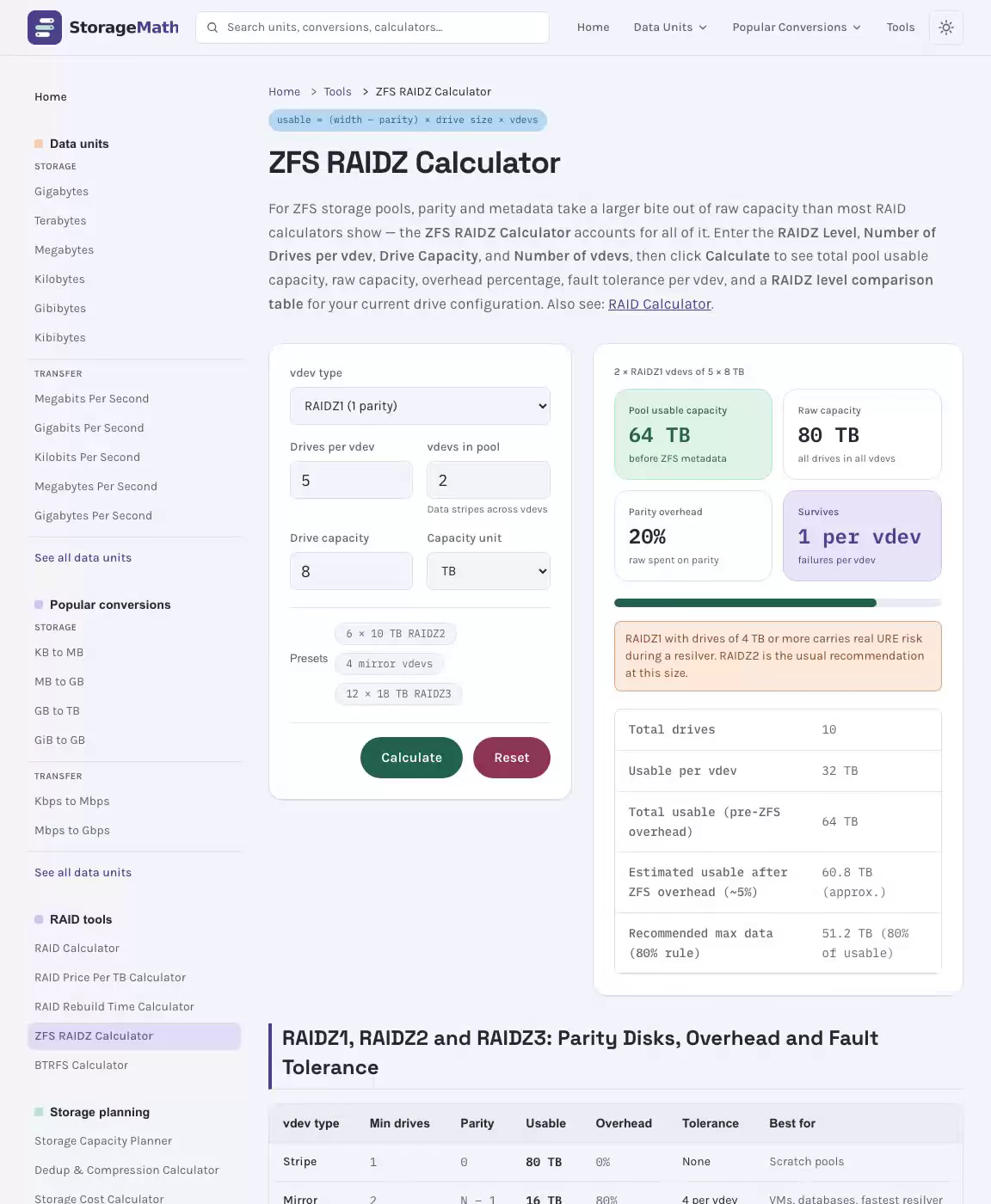
2 × RAIDZ1 vdevs of 5 × 8 TB
Results
Pool usable capacity
before ZFS metadata
Raw capacity
all drives in all vdevs
Parity overhead
raw spent on parity
Survives
failures per vdev
RAIDZ1 with drives of 4 TB or more carries real URE risk during a resilver. RAIDZ2 is the usual recommendation at this size.
| Total drives | 10 |
| Usable per vdev | 32 TB |
| Total usable (pre-ZFS overhead) | 64 TB |
| Estimated usable after ZFS overhead (~5%) | 60.8 TB (approx.) |
| Recommended max data (80% rule) | 51.2 TB (80% of usable) |
RAIDZ1, RAIDZ2 and RAIDZ3: Parity Disks, Overhead and Fault Tolerance
| vdev type | Min drives | Parity | Usable | Overhead | Tolerance | Best for |
|---|---|---|---|---|---|---|
| Stripe | 1 | 0 | 80 TB | 0% | None | Scratch pools |
| Mirror | 2 | N − 1 | 16 TB | 80% | 4 per vdev | VMs, databases, fastest resilver |
| RAIDZ1 | 3 | 1 | 64 TB | 20% | 1 per vdev | General storage, low cost |
| RAIDZ2 | 4 | 2 | 48 TB | 40% | 2 per vdev | Large drives, NAS |
| RAIDZ3 | 5 | 3 | 32 TB | 60% | 3 per vdev | Archive, highest redundancy |
How ZFS Allocates Capacity Across vdevs, Drives and Parity
Planning a ZFS storage array without knowing your real available capacity is like buying a house without measuring the rooms — the numbers on paper rarely match what you can actually use. This ZFS RAIDZ Calculator gives you a precise, ZFS-aware usable capacity estimate before you spend a single dollar on units, helping you compare array types, understand protection overhead, account for reserved space, and convert between binary and decimal units so your capacity planning decisions are grounded in reality rather than manufacturer marketing figures. Whether you are building a home lab NAS, scaling server storage, or configuring a TrueNAS array, the results here reflect how the file system actually allocates and reserves space on your pool.
See the ZFS RAIDZ Calculator in Action
ZFS & RAIDZ Pool Capacity Calculator — Understanding Your Results
The ZFS / RAIDZ Capacity Calculator above accepts the following key inputs and produces a layered breakdown of your array's allocation from raw volume down to the space you can actually write data to. Here is what each field and output means for your real-world server storage setup:
- RAID type: Select from RAIDZ1 (single protection, variable stripe width), RAIDZ2 (double protection), RAIDZ3 (triple protection), mirror (two-way equivalent to RAID1/RAID10), or stripe (RAIDZ0, no redundancy). Each choice directly controls storage overhead and resilience.
- Drive capacity: Enter the dimension of each unit in gigabytes or terabytes as marked by the manufacturer — that is, powers of 10 (decimal). The calculator converts this to tebibytes internally, because the file system operates using binary (powers of 2) units.
- Drive sector size: Choose 512 B (
ashift=9) for legacy units or 4 KiB (ashift=12) for modern hard disks and SSDs. The ashift value is set at array creation and cannot be changed afterward, so choose carefully. The sector size overhead introduced by mismatched ashift settings can severely degrade throughput. - Drives per RAID group: The count of units per virtual device (top-level virtual device). For RAIDZ arrays, this is the stripe width — for example, 6 units per RAIDZ2 virtual device.
- Number of RAID groups: How many virtual devices make up your array. Multiple groups stripe data across virtual devices, increasing both capacity and throughput.
- ZFS record size: The maximum zfs recordsize for your datasets. The default is 128 KiB (a 128 KiB record), but usage patterns like databases may benefit from specific tuning to a smaller block dimension. Choosing the right zfs recordsize for your workload affects both space efficiency and read throughput.
- % free space limit: The recommended array fill level — keeping at least 20% free is strongly advised to maintain best throughput, prevent fragmentation, and give the system adequate room for metadata and copy-on-write operations. Expressed in decimal places for precision.
- Single drive cost: Optional monetary cost per unit, used only to calculate total cost and cost per usable unit. It has no impact on capacity calculations.
The calculator outputs four progressively refined capacity figures. Total number of drives: simply the product of drives per RAID group and number of RAID groups — your total unit count. Zpool storage capacity: raw volume minus the loss for drive partitioning, on-disk structure such as virtual device labels (4.5 MiB labels per device), the boot loader region, labels, and metaslab allocation boundaries — but before protection data is deducted. This figure is close to what zpool list shows under SIZE. ZFS usable storage capacity deducts the protection and padding reservation plus the slop space allocation, and corresponds closely to the sum of USED and AVAIL shown by zfs list. Finally, practical usable capacity deducts your chosen % free space limit to show the space you should actually treat as available for data. All results are displayed in both (TiB) (tebibytes, binary) and (TB) (terabytes, decimal), along with a (%) column showing each layer as a proportion of total raw capacity.
ZFS RAIDZ Calculator — RAIDZ Configuration Reference: Usable Capacity, Protection, and Resilience
Choosing the right array type is the single biggest lever on your configuration's capacity efficiency and resilience characteristics. The table below compares all supported array types in this free zfs raidz array tool, showing minimum units, protection drives lost per virtual device, the usable capacity formula, and the fault tolerance of each configuration. Use this as a quick configuration guide before entering your specific parameters above.
| RAID Type | Min Drives | Parity Drives Lost per vdev | Usable Capacity Formula | Fault Tolerance | Typical Capacity Efficiency |
|---|---|---|---|---|---|
| RAIDZ0 (Stripe) | 1 | 0 | C_(usable) = n × D | None — any unit failure = data loss | 100% |
| Mirror (RAID1 / RAID10) | 2 | n/2 drives | C_(usable) = (n)/(2) × D | Single-disk fault tolerance per mirror group; best performance | 50% capacity efficiency |
| RAIDZ1 (RAID-Z1) | 3 | 1 | C_(usable) = (n - 1) × D | Single-disk fault tolerance; single protection stripe | Good capacity efficiency (~80–92%) |
| RAIDZ2 (RAID-Z2) | 4 | 2 | C_(usable) = (n - 2) × D | Double-disk fault tolerance; double protection stripe | Balanced capacity and protection |
| RAIDZ3 (RAID-Z3) | 5 | 3 | C_(usable) = (n - 3) × D | Triple protection; maximum fault tolerance | Good capacity efficiency at large widths |
| dRAID2 | Varies | 2 per protection group | See dRAID section below | Double-disk fault tolerance; faster rebuild | Varies by group width and spares |
For a mirror group, the file system implements a two-way arrangement where each piece of data is written to all units in the group simultaneously, giving you the best read throughput and single-disk fault tolerance — at the cost of 50% capacity efficiency. Mirrored groups are equivalent to RAID1 for two units, or RAID10 when you stripe multiple mirror groups. Striped arrays (RAIDZ0) have no protection data and no check blocks, so any single unit failure results in total data loss — they are appropriate only for scratch or cache workloads where data protection is not required.
How ZFS Pool Capacity Is Calculated Using This ZFS Capacity Calculator
Understanding the math behind your array's capacity lets you make smarter decisions during planning and helps you interpret the layered output this calculator produces. The file system calculates allocation at multiple levels: physical volume, logical virtual device address space, array-level allocatable space, and finally the space visible to datasets. Each layer subtracts a different category of overhead — drive partitioning loss, protection reservation, reserved buffer space, and free space reservation. Let's walk through every layer in detail. Related: Cloud Storage Cost Calculator.
Step 1 — From Raw Volume to Zpool Storage Capacity
Your unit capacity is expressed in decimal terabytes (powers of 10) by manufacturers. Because the file system reports dimension in binary units, the calculator converts each unit's rated size to tebibytes using the conversion factor:
1 TiB = 2⁴⁰ bytes ≈ 1.099511627778 TBSo a unit marketed as 10 TB actually provides approximately 10 ÷ 1.099511627778 ≈ 9.094947 TiB of binary capacity. This gap between decimal and binary units is why your array's dimension always looks smaller than the sum of your units' rated sizes — and it is the first reason a capacity estimator like this one is essential for accurate capacity planning.
The total raw storage capacity is simply:
C_(raw) = n_(drives) × D_(TiB)where n_(drives) is the total number of units (drives per RAID group × number of RAID groups) and D_(TiB) is the per-unit capacity in binary units. From this aggregate figure, the system subtracts overhead for the on-disk structure of each virtual device — specifically, label space (four labels per device, each 256 KiB, placed at known offsets), a boot loader region at the front of the volume, and the padding sectors needed so that the usable address space aligns to a metaslab boundary. This produces the zpool storage capacity — the pool asize — which is what zpool list reports as SIZE. The aggregate minus this partitioning and metaslab allocation overhead gives you a number very close to, but slightly less than, the sum of raw unit sizes.
The file system divides each virtual device's address space into metaslabs — the fundamental unit of space allocation. The count of metaslabs (ms_count) per device is determined by the ms_shift value, which sets metaslab dimension. Each metaslab has its own space map (spacemaps) tracking free and consumed regions. The vdev_deflate_ratio (deflate ratio) accounts for the fact that not all logical blocks map 1:1 to physical sectors — for example, on a RAIDZ device, a logical block maps to a variable stripe width including check sectors, so the asize of a block is larger than its logical dimension. The array-level deflate ratio is used by zpool list to show the compression factor and correct for this when reporting USED.
Step 2 — Protection and Padding Reservation Across RAIDZ Levels
Once you have the zpool storage capacity, the next deduction is the reservation for parity and padding. This is the core of what makes RAIDZ different from legacy array configurations: the file system uses a variable stripe width, meaning each write can occupy a different number of data sectors depending on the dimension of the data being written. Check sectors are computed per stripe, not per fixed-width block. This variable block approach is one of the most powerful features of the file system — it avoids the read-modify-write penalty common in traditional RAID — but it means the effective protection overhead across the array is not simply (1)/(n) of raw capacity.
The reservation for parity and padding is calculated using the method described by Matt Ahrens in the RAIDZ stripe width analysis. For a given RAIDZ level with nparity protection drives per device and a device width of w drives, the worst-case protection cost across an array full of blocks is determined by the ZFS record size (recordsize) relative to the stripe width. The key formula for check overhead per stripe, for a single level, is:
For raidz1 (RAID-Z1): 1 protection drive per group — cost scales as (1)/(w).
For raidz2 (RAID-Z2): 2 protection drives lost — cost scales as (2)/(w).
For a triple-protection configuration: 3 protection drives lost — cost scales as (3)/(w).
Padding sectors are also included in this reservation — partial stripe writes cause alignment loss, particularly when a record does not fill a complete stripe. The protection level directly determines your array's resilience: RAID-Z1 provides single-disk fault tolerance, RAID-Z2 provides double-disk fault tolerance, and a triple-protection setup means up to three simultaneous unit failures can be survived. This protection and padding reservation is not applicable to mirror groups, where data recovery works differently through full data duplication.
Step 3 — ZFS Slop Space and Its Impact on Usable Allocation
After deducting protection costs, the file system reserves an additional block called the slop space allocation (sometimes called spa slop or zfs slop). This is an internal reservation that ensures the array can always complete in-flight transactions, write metadata, and perform administrative operations even when the array appears nearly full. Without this buffer, a completely filled array could deadlock — the system needs room to write new data pointers, space maps, and the MOS configuration even during a delete operation. This zfs overhead directly impacts how much space you can treat as available.
The zfs slop calculation is:
In plain terms: the system reserves 1/32 of array capacity as a buffer, subject to a minimum of 128 MiB and a maximum cap of 128 GiB. For most practical array sizes, this buffer is simply , which is roughly 3.125% of array capacity. This buffer is why your array appears to run out of room before it is technically 100% full — and why the estimator deducts it before displaying usable allocation figures. The storage overhead from this reservation is a key part of accurate capacity planning.
The ZFS usable storage capacity is therefore:
This figure corresponds closely to USED + AVAIL as reported by the dataset list command. Running zpool list will show the array dimension and consumed values, while the dataset list view shows the dataset-level breakdown. The annual failure rate and data recovery considerations mean you should always maintain a meaningful free buffer — not just rely on the internal buffer alone.
Step 4 — Recommended Free Space Limit and Practical Usable Capacity
The % free space limit field represents the minimum free array space you want to maintain at all times. Throughput degrades noticeably as array fill levels rise above 80%, because the allocator has fewer metaslabs to choose from and must perform more fragmented allocations. The recommended fill level is to keep at least 20% free. Setting this field to 20 means the calculator deducts 20% of ZFS usable storage capacity to give you practical usable capacity — the number you should actually plan your data around.
Keeping free space available also matters for data recovery: when a unit fails and the system begins a resilver operation, it needs to read every allocated block and recompute protection data onto the replacement volume. A fuller array means more data to rebuild, longer resilver time, and a longer window of exposure where a second unit failure would be catastrophic. Setting your minimum spares count and monitoring array fill levels through zpool list are both critical parts of responsible array design.
Worked Examples: ZFS Capacity Calculation Step by Step
Example 1 — 6 × 10 TB Drives in RAIDZ2: Capacity and Efficiency
This is the most common configuration for a balanced home lab or small NAS — a single RAIDZ2 virtual device with 6 units, giving you double-disk fault tolerance at a reasonable cost per usable binary unit. Here is the full calculation walkthrough, showing every layer from aggregate raw capacity down to practical usable space: See also: RAID Rebuild Time Calculator.
- Convert unit capacity from decimal to binary: 10 TB ÷ 1.099511627778 ≈ 9.094947 TiB per unit
- Total raw storage capacity: 6 × 9.094947 = 54.569 TiB (approximately 60.000 TB)
- Zpool storage capacity after partitioning and metaslab alignment: Approximately 54.375 binary units (99.64% of raw — subtracts label overhead, skip sectors, and padding sectors for metaslab boundary alignment)
- Protection reservation (RAIDZ2, 2 check drives out of 6): Approximately 2 units' worth = (2)/(6) ≈ 33.33% overhead on the data sectors, yielding approximately 36.25 binary units of array usable capacity
- Slop space allocation (1/32 of array): 54.375 ÷ 32 ≈ 1.699 TiB
- ZFS usable storage capacity: 36.25 - 1.699 ≈ 34.55 TiB (approximately 37.99 TB)
- Capacity efficiency: (34.55)/(54.569) ≈ 63.3% of total raw capacity — or approximately 77.11% of zpool storage capacity after accounting for protection and buffer
For the specific 5-unit RAIDZ1 reference configuration (5 units at 0.5 TB each) used to calibrate this calculator, the output table data shows: raw storage capacity 2.500000 TB / 2.273737 binary units; zpool storage capacity 2.491081 TB / 2.265625 binary units (99.64%); ZFS usable storage capacity 1.927760 TB / 1.753287 binary units (77.11%). These specific conversion values — 1.753287 binary units and 1.927760 TB for ZFS usable, and 2.265625 binary units and 2.491081 TB for array capacity — appear in the calculator output and confirm that the binary conversion and buffer deduction are both being applied correctly. The results are shown to the appropriate number of decimal places for precision.
| Capacity Layer | Value (TiB) | Value (TB) | % of Raw |
|---|---|---|---|
| Total raw storage capacity (6 × 10 TB) | 54.569 | 60.000 | 100% |
| Zpool storage capacity (after partitioning) | 54.333 | 59.727 | ~99.6% |
| Protection and padding reservation (RAIDZ2, 2 of 6) | −18.111 | −19.909 | ~33.3% |
| Zpool usable storage capacity | 36.222 | 39.818 | ~66.4% |
| Slop space allocation (1/32) | −1.697 | −1.866 | ~3.1% |
| ZFS usable storage capacity | 34.525 | 37.952 | ~63.3% |
| Practical usable (20% free reserved) | 27.620 | 30.362 | ~50.6% |
Example 2 — 8 × 4 TB Drives in RAIDZ1 Across Two RAID Groups of 4
Using two RAID groups (two top-level virtual devices) instead of one changes both resilience and the cost structure. Here, each virtual device is a RAIDZ1 group of 4 units (4 KiB sector drives, so ashift=12). This array layout stripes data across both groups, roughly doubling write throughput compared to a single virtual device.
- Unit capacity: 4 TB = 4 ÷ 1.099511627778 ≈ 3.638 TiB
- Total raw capacity: 8 × 3.638 = 29.103 TiB (32.000 TB)
- Per-group protection loss (RAIDZ1, 1 of 4 units): (1)/(4) = 25% cost per group
- Array usable after protection across both groups: ≈ 21.777 TiB
- Buffer space: ≈ 0.906 TiB
- ZFS usable storage capacity: ≈ 20.871 TiB (22.959 TB)
- Practical usable (20% free): ≈ 16.697 TiB
- Array capacity efficiency: approximately 71.7% of raw capacity — better than a mirror group's 50% capacity efficiency, worse than a wider RAIDZ2 at high unit counts
With a single unit cost of $80 per unit (8 × $80 = $640 total cost), and approximately 20.871 binary units of ZFS usable storage capacity, the cost per binary unit usable is approximately $30.67 — significantly more cost effective than a mirror configuration using the same 8 units, which would yield only 14.55 binary units usable at $44.00 per binary unit. This illustrates why a capacity calculator is so valuable: comparing these options side by side before committing to an array configuration can save substantial money. The annual failure rate for two RAIDZ1 groups is also worth evaluating — with a unit failure rate of 1–2%, losing one unit per group during the rebuild window is a real risk, which is why RAIDZ2 is commonly recommended for production setups.
Example 3 — 12 × 18 TB Drives in RAIDZ3 (Enterprise Storage Configuration)
For a high-capacity enterprise hardware array with maximum fault tolerance, a single RAIDZ3 virtual device of 12 units using 18 TB volumes and 4 KiB sector drives (ashift=12, or ashift 12) is a common enterprise architecture. This configuration is typical in TrueNAS Enterprise setups and large server storage installations where data protection and resilience are the top priorities.
- Unit capacity: 18 TB volumes = 18 ÷ 1.099511627778 ≈ 16.371 TiB per unit
- Total raw capacity: 12 × 16.371 = 196.450 TiB (216.000 TB)
- Protection loss (RAIDZ3, 3 of 12 units): (3)/(12) = 25% overhead
- Array usable after protection and padding: ≈ 147.337 TiB
- Buffer space (capped at 128 GiB for very large arrays): 128 GiB = 0.125 binary units
- ZFS usable storage capacity: ≈ 147.212 TiB (161.845 TB)
- With 20% % free space limit: practical usable ≈ 117.770 TiB
- Capacity efficiency: approximately 74.9% — good capacity efficiency for triple protection, especially at 12 units per group
Selecting ashift=12 for these 18 TB volumes is critical. Modern 18 TB hard disks use 4 KiB physical sectors. If you set ashift=9 (treating them as 512 B sector volumes), the file system will perform write alignment to 512-byte logical block addresses that are misaligned to the physical 4 KiB sector of the volume — causing a severe read-modify-write penalty on every partial write, degrading throughput, and reducing efficiency. Using ashift=12 ensures the file system writes in 4 KiB minimum block multiples, aligned to the physical sector size of the volume. The sector size overhead from a mismatched ashift setting is one of the most common and avoidable configuration mistakes. For 12 units of 18 TB in a triple-protection setup (a 14-unit 18 TB arrangement is another common enterprise configuration), the parameters and group layout follow identical logic.
dRAID Capacity Calculation and the dRAID Capacity Calculator
How dRAID Differs from Standard RAIDZ in Usable Allocation and Rebuild Behaviour
dRAID is a distributed array variant introduced in OpenZFS designed specifically for arrays with numerous units — typically more than 100 hard disks — where the primary concern is faster data recovery rather than maximising raw capacity. Standard RAIDZ recovery requires resilvering an entire virtual device's worth of data through a single replacement volume, which can take many hours or even days at petabyte scales. dRAID distributes the rebuild workload across all units in the group, achieving reduced resilver time by parallelising the rebuild operation.
The dRAID capacity calculation differs from standard RAIDZ in several important ways:
- Group width and protection group: dRAID divides the array into fixed-width protection groups (group width = data units + check units + spares). The available capacity depends on the group alloc dimension and how many units are designated as distributed spares. The redundancy group structure is central to how dRAID manages both capacity and resilience.
- dRAID reflow and reflow space: dRAID supports online expansion — adding units triggers a redistribution that spreads data across the new volumes. The reflow space reserved for this operation slightly reduces immediately available capacity.
- Minimum allocation dimension and row height: dRAID allocates in fixed row height multiples (a 16 MiB row is common), which affects how the minimum allocation dimension interacts with the ZFS record size. This can cause alignment loss between rows and metaslab boundaries, computed using the least common multiple (lcm) and greatest common divisor (gcd) of the row height and the recordsize value — a closed-form equation approach described in the OpenZFS documentation.
- Fast dRAID calculation mode: The dRAID capacity calculator on this page supports a fast calculation mode that approximates the complex period alignment and alignment pattern losses without iterating through every possible stripe configuration, making the calculation practical for large arrays with numerous units.
For a dRAID2 configuration (double protection, equivalent to RAIDZ2 in fault tolerance) with 20 data units, 2 check units, and 2 distributed spares per protection group across a 24-unit virtual device, the effective usable capacity is approximately:
In this example: (20)/(20 + 2 + 2) = (20)/(24) ≈ 83.3% of raw capacity is data, before buffer and other deductions. The minimum spares count and device children count directly affect this ratio. Compared to a standard RAIDZ2 with 22 data units + 2 check units (no dedicated spares), dRAID2 has slightly lower capacity efficiency — the trade-off for fast data recovery. Using the dRAID capacity calculator fields above, you can model this trade-off directly, comparing dRAID results to RAIDZ results for the same unit count and volume dimension to determine which array layout best matches your usage patterns and resilience requirements.
The zdb command can be used post-creation to inspect internal array metrics including device asize, array asize, metaslab dimension, metaslab count (ms_count), ms_shift, and the show deflate ratio output — verifying that your real array matches the capacity reservation predicted by this calculator. For environments using FreeBSD or TrueNAS Core, a 2 GiB swap partition (disk swap size, or 2 GiB swap) is typically reserved per unit during array creation, which also reduces available device raw dimension slightly — this drive partitioning is accounted for in the calculator's zpool storage capacity figure through the osize and device asize calculation.
Whether you are doing capacity planning for a new home lab file system, scaling out server storage with expansion shelf planning, or comparing legacy array alternatives for your organisation's file storage infrastructure, understanding every layer of ZFS capacity calculation — including zfs overhead and how it affects your zfs raidz array — helps you avoid costly surprises and make the best use of every gigabyte. Use this online calculator as your first step in array planning, then validate your expected capacity reservation and array metrics against live output once your configuration is running. For deeper concepts and hands-on education, including webinars and a downloadable guide, resources from the open-source community — including OpenZFS documentation, the ZFS primer, and infrastructure guides from ix systems and other contributors — provide the configuration depth needed to tune your arrays for specific usage patterns, data integrity requirements, and long-term goals.
ashift, Sector Alignment and ZFS Pool Expansion Caveats
ashift Setting: ZFS ashift should match the physical sector size of your drives: ashift=9 for 512-byte sectors, ashift=12 for 4K native drives (most modern HDDs and SSDs). Wrong ashift causes write amplification — set it correctly at pool creation as it cannot be changed later.
80% Rule: Never fill a ZFS pool beyond 80% capacity. ZFS uses copy-on-write and needs free space for its block allocator to work efficiently. Above 80%, fragmentation causes severe write performance degradation on spinning media.
Snapshot Space: ZFS snapshots share blocks with the live filesystem. As data changes, snapshots grow. A heavily snapshotted pool can silently fill to capacity even when apparent data usage appears low.
RAIDZ vs Mirror: Mirror vdevs offer significantly better random read and rebuild performance than RAIDZ. RAIDZ offers better capacity efficiency. For databases and VMs, mirror vdevs are preferred. For archival NAS, RAIDZ2 is preferred.
dRAID: OpenZFS 2.1+ introduces dRAID, a distributed spare RAIDZ variant that enables faster rebuilds by spreading the hot spare across all drives in the vdev, enabling parallel rebuild. Use dRAID for large vdevs with many drives.
ZFS RAIDZ Calculator: Frequently Asked Questions
3 questions Quick answers about the ZFS RAIDZ Calculator and how its results are calculated.
-
How do I calculate ZFS RAIDZ usable capacity?
For a single RAIDZ vdev: usable = (drives_per_vdev - parity_drives) × drive_size. RAIDZ1 uses 1 parity drive, RAIDZ2 uses 2, RAIDZ3 uses 3. For a pool with multiple vdevs, multiply usable_per_vdev by the number of vdevs.
-
What is the optimal number of drives per RAIDZ vdev?
For best read performance, use power-of-2-plus-parity: RAIDZ1: 3, 5, 9 drives. RAIDZ2: 4, 6, 10 drives. RAIDZ3: 5, 7, 11 drives. Larger vdevs reduce parity overhead but increase rebuild time and risk.
-
What is the difference between ZFS RAIDZ and traditional RAID 5?
ZFS RAIDZ uses variable-width stripes that eliminate the RAID-5 write hole, provides end-to-end data integrity checking via checksums, and integrates with the ZFS copy-on-write filesystem. Traditional RAID 5 requires NVRAM to protect against partial stripe writes during power failures.