

NVMe Queue Depth Calculator
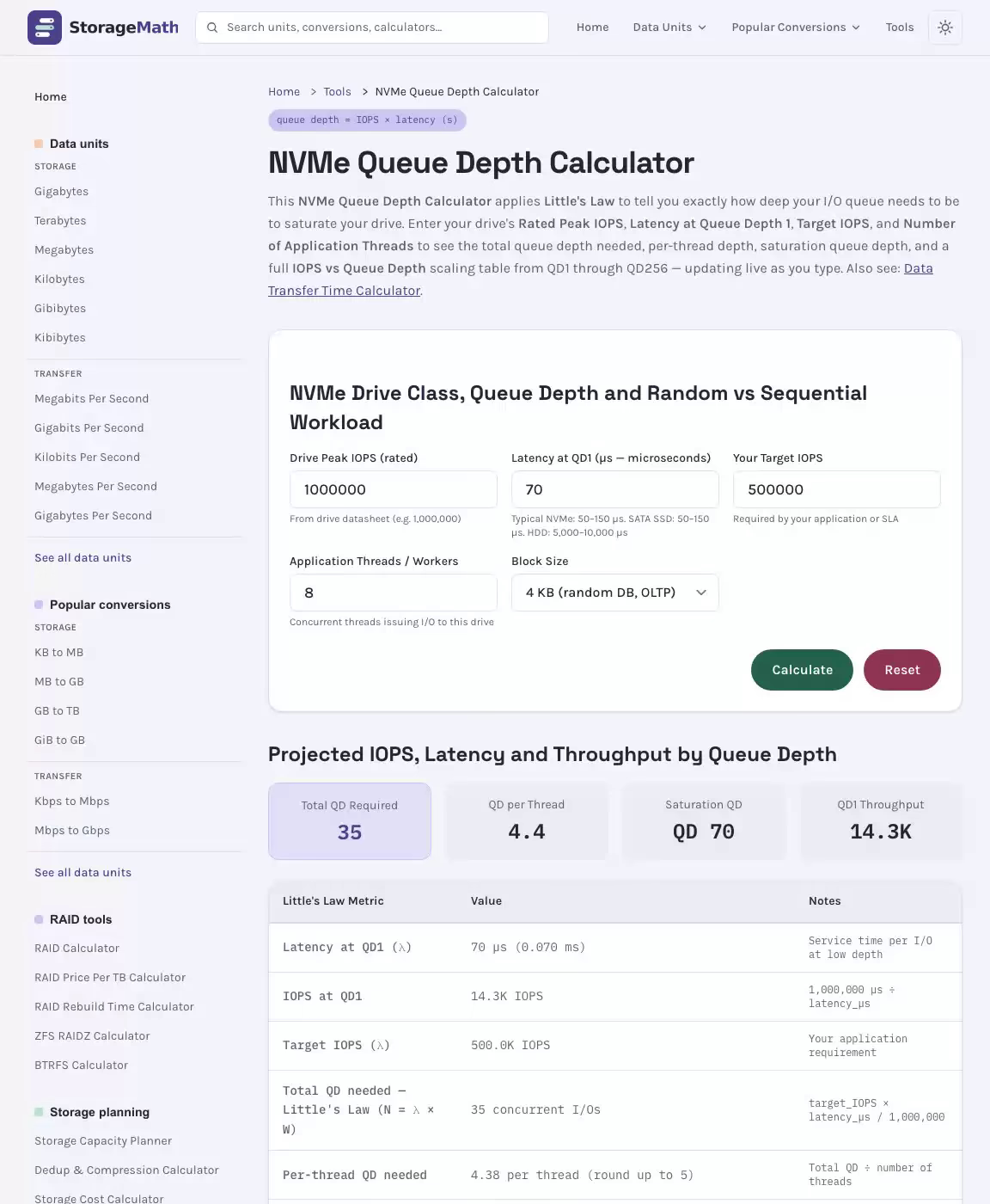
This NVMe Queue Depth Calculator applies Little's Law to tell you exactly how deep your I/O queue needs to be to saturate your drive. Enter your drive's Rated Peak IOPS, Latency at Queue Depth 1, Target IOPS, and Number of Application Threads to see the total queue depth needed, per-thread depth, saturation queue depth, and a full IOPS vs Queue Depth scaling table from QD1 through QD256 — updating live as you type. Also see: Data Transfer Time Calculator.
NVMe Drive Class, Queue Depth and Random vs Sequential Workload
Projected IOPS, Latency and Throughput by Queue Depth
Total QD Required
QD per Thread
Saturation QD
QD1 Throughput
| Little's Law Metric | Value | Notes |
|---|---|---|
| Latency at QD1 (λ) | 70 µs (0.070 ms) | Service time per I/O at low depth |
| IOPS at QD1 | 14.3K IOPS | 1,000,000 µs ÷ latency_µs |
| Target IOPS (λ) | 500.0K IOPS | Your application requirement |
| Total QD needed — Little's Law (N = λ × W) | 35 concurrent I/Os | target_IOPS × latency_µs / 1,000,000 |
| Per-thread QD needed | 4.38 per thread (round up to 5) | Total QD ÷ number of threads |
| Saturation queue depth (peak IOPS) | QD 70 (70.0 exact) | QD at which drive reaches rated peak IOPS |
| Throughput at target IOPS + block size | 1.95 GB/s (500.0K × 4 KB) | target_IOPS × block_size |
| Can your threads saturate the drive? | ✗ No — 8 threads × QD5 = 40 I/Os < saturation QD 70. Add more threads or increase per-thread QD. | threads × per-thread QD ≥ saturation QD? |
Estimated IOPS vs Queue Depth Scaling
| Queue Depth | Estimated IOPS | % of Peak | Throughput (MB/s) | Est. Latency (µs) | Status |
|---|---|---|---|---|---|
| QD 1 | 14.3K | 1% | 56 MB/s | 70 µs | 1% of peak |
| QD 2 | 28.6K | 3% | 112 MB/s | 70 µs | 3% of peak |
| QD 4 | 57.1K | 6% | 223 MB/s | 70 µs | 6% of peak |
| QD 8 | 114.3K | 11% | 446 MB/s | 70 µs | 11% of peak |
| QD 16 | 228.6K | 23% | 893 MB/s | 70 µs | 23% of peak |
| QD 32 | 457.1K | 46% | 1.79 GB/s | 70 µs | 46% of peak |
| QD 64 | 914.3K | 91% | 3.57 GB/s | 70 µs | 91% of peak |
| QD 128 | 1.000M | 100% | 3.91 GB/s | 128 µs | Saturated |
| QD 256 | 1.000M | 100% | 3.91 GB/s | 256 µs | Saturated |
⚠ Your current thread count (8 threads × QD5) cannot fully saturate the drive. You need QD70 total to reach peak IOPS. Increase threads, per-thread queue depth, or use async I/O.
Note: SATA AHCI (max QD=32) cannot reach saturation for this drive. NVMe with its multi-queue architecture is required.
NVMe vs SATA vs SAS Queue Architecture
| Interface | Protocol | Max Queues | Depth per Queue | Max Outstanding I/Os | Multi-core Scaling |
|---|---|---|---|---|---|
| SATA SSD / HDD | AHCI | 1 | 32 | 32 | Poor — single shared queue |
| SAS HDD / SSD | SCSI | 1 per initiator | 254 | 254 | Limited — one queue per HBA port |
| NVMe SSD (PCIe) | NVMe 1.x | 65,535 | 65,535 | 4.29 billion | Excellent — one queue per CPU core |
| NVMe-oF (RDMA) | NVMe 1.x | 65,535 | 65,535 | 4.29 billion | Excellent + network fabric latency |
In practice, NVMe drives support 2–128 queues depending on firmware implementation. The spec allows 65,535 but real devices expose fewer queues tuned to their internal parallelism. Linux NVMe driver maps one submission queue per CPU core by default.
Typical NVMe Latency & IOPS by Device Class
| Drive Class | QD1 Latency (µs) | Peak IOPS (4K random) | Saturation QD | Interface |
|---|---|---|---|---|
| Consumer NVMe (Gen 3) | 70–120 | 350K–550K | ~32–64 | PCIe 3.0 x4 |
| High-end Consumer (Gen 4) | 50–80 | 700K–1,000K | ~64–128 | PCIe 4.0 x4 |
| Enterprise Read-Int. (Gen 4) | 80–120 | 800K–1,500K | ~128–256 | PCIe 4.0 x4 |
| Enterprise Write-Int. (Gen 4) | 70–100 | 500K–800K | ~64–128 | PCIe 4.0 x4 |
| Consumer NVMe (Gen 5) | 40–70 | 1,500K–2,000K | ~128–256 | PCIe 5.0 x4 |
| Intel Optane P5800X | 6–10 | 1,500K | ~16–32 | PCIe 4.0 x4 |
| SATA SSD (reference) | 70–100 | 90K–100K | ~32 | SATA 6Gb/s |
Why Queue Depth Multiplies NVMe IOPS and Reduces Latency
When your data storage stack isn't delivering the predictable response times your applications demand, the answer often lies in a single parameter: queue depth. The NVMe Queue Depth Calculator gives you a mathematically grounded starting point — translating your measured delay and target IOPS into a concrete iodepth value — so you stop guessing and start tuning with confidence. Whether you're chasing tight p99 response rates for a delay-sensitive datastore or pushing peak data transfer through a pipeline, getting your queue depth choices right is the difference between a system that scales and one that silently degrades.
See the NVMe Queue Depth Calculator in Action
How NVMe Queue Depth Mechanics Actually Work Under the Hood
Understanding how NVMe queuing mechanics shape i/o performance requires looking inside the protocol itself. Unlike legacy SCSI commands carried over older SAN interconnects, NVMe was designed from the ground up for parallelism. At its core, the protocol exposes a set of submission queues and completion queues — paired rings in host memory that the NVMe driver uses to post and retire I/O requests without serializing through a single command path. Each queue pair can be pinned to a CPU core, and the multi-queue block layer in the OS dispatches I/O across those pairs to minimize lock contention and reduce kernel overhead.
The queue depth formula that connects these mechanics to real numbers is elegantly simple:
Queue Depth = Latency (sec) × IOPSThis queue depth equation — sometimes called the Little's Law application for storage networking — tells you exactly how many pending commands must be outstanding at any moment to sustain a given IOPS rate at a given system performance target. If you need 40,000 operations per second with a completion delay of 3 milliseconds, the needed queue depth is:
Queue Depth = 40,000 × 0.003 = 120Similarly, achieving 20,000 operations per second at a 4-millisecond processing time requires a queue depth of 80. This iops equation is your baseline before any performance testing begins.
# Core queue depth formula
Queue Depth = Latency (sec) x IOPS

# Example: 40k write IOPS at 3ms latency
Queue Depth = 40000 x 0.003 = 120

# Example: 20k write IOPS at 4ms latency
Queue Depth = 20000 x 0.004 = 80
SQ/CQ Sizing and Host-Side iodepth Interaction
Effective queue depth tuning isn't just about setting iodepth higher in your benchmark tool. The actual in-flight capacity is bounded by sq/cq sizing — the submission queue and completion queue ring buffer depths negotiated during controller initialization. If your host-side iodepth exceeds what the SQ/CQ pipeline can service, you create host-side queuing before the command even reaches the NVMe media. That hidden buffering inflates tail delay, turning what looks like a data-rate gain into a p99 latency disaster. Always validate with p99 delay profiles and completions-per-second metrics, not IOPS alone.
The distinction between iodepth and numjobs is equally important. iodepth controls how many outstanding I/O requests a single fio job maintains — it stresses the device queues directly. numjobs creates additional parallel submitters, which changes CPU scheduling, softirq distribution, and thread contention patterns across cores. Many tasks scale better with modest iodepth and more jobs until cpu saturation becomes the limiter. Treat them as separate levers: one pressures the drive controller, the other pressures the host submission and completion path.
The Latency Knee Point and Why It Defines Your Queue Depth Budget
Every NVMe device has a latency knee point — the inflection point where adding more queue depth stops increasing output meaningfully and starts accelerating p99 tail delay. Below this point, higher depth fills the device pipeline efficiently, improving device utilization and peak iops. Beyond it, you are simply storing more work in the system: the drive controller, the I/O layer, or the CPU becomes the bottleneck, and every additional pending command contributes to queueing delay rather than useful work.
The latency knee point is not a fixed value — it shifts depending on task type, read/write mix, block size, and whether you are accessing locally attached NVMe or a network-attached volume across the network. This is why a queue depth sweep during baseline creation is essential: you cannot determine your queue depth budget from the formula alone. The equation tells you the theoretical minimum depth to sustain your IOPS target; the test tells you whether the device can absorb that depth without inflating delay profiles.
The NVMe/TCP impact deserves special attention here. When your NVMe data storage is accessed over an Ethernet network — whether through NVMe over fabrics (NVMe-oF) or NVMe over TCP specifically — the host pays for tcp processing, packet scheduling, and buffer management on top of NVMe command handling. Network RTT becomes a first-class constraint alongside processing time on the SSD itself. This typically means optimal queue depth for NVMe/TCP is lower per connection than for locally attached NVMe, with parallelism achieved by scaling out initiators and adding connections rather than piling on more pending commands per queue. Excessive depth over NVMe/TCP transport amplifies in-flight buffering, increases cpu cost per I/O, and worsens delay jitter during microbursts, retransmits, or network congestion.
For SPDK-based or other user-space NVMe-oF targets, the tuning profile shifts again. By moving the data-plane processing out of the kernel, you eliminate context switching and reduce irq noise, which lets you sustain the same data rate at a lower effective queue depth. This matters most when you need predictable response across a fleet rather than peak output on a single node — a common requirement in container-orchestrated environments and cloud-native platforms where task concurrency fluctuates with pod placement.
Using the NVMe Queue Depth Calculator for Your Specific Workload: Three Real-World Examples
The calculator above gives you an instant recommendation, but understanding how those numbers behave under real conditions requires walking through concrete examples. Below are three worked scenarios covering the most common cases teams encounter when tuning NVMe performance. Related: Deduplication & Compression Calculator.
Achieving High IOPS at Low Queue Depth in VMware and Container Platform Environments
Some applications — particularly desktop virtualization, SMB CAD/CAM tasks, manufacturing ERP systems, and certain OLTP relational engines — require high i/o at low queue depth. These are delay-sensitive tasks where predictable commit timing and read response rates matter more than raw data transfer capacity. This is a well-documented challenge in vmware environments, and it remains equally relevant after vmware migration to a container platform or a hyperconverged deployment.
Use Case 1 – 20k write IOPS at queue depth of 8:
You need 20,000 write IOPS. Your measured steady-state delay under light load is 400 microseconds (0.0004 seconds). The formula predicts:
Queue Depth = 20,000 × 0.0004 = 8A queue depth of 8 should theoretically sustain this rate. Validate with fio:
fio --name=write_iops_test \
    --ioengine=libaio \
    --rw=randwrite \
    --bs=4k \
    --iodepth=8 \
    --numjobs=4 \
    --runtime=120 \
    --time_based \
    --group_reporting \
    --filename=/dev/nvme0n1
If your fio output shows IOPS near 20k with p99 delay under 1ms, you are operating below the latency knee point — ideal for delay-sensitive data engines. If p99 exceeds your latency SLO, reduce iodepth to 4 or 6 and re-test. If output falls short of 20k IOPS, your device needs a slightly higher depth, meaning actual processing time is longer than your light-load measurement suggested.
Use Case 2 – 40k write IOPS at queue depth of 4:
This scenario demonstrates how lower depth combined with higher drive parallelism — more numjobs, more NVMe SSDs, or disaggregated capacity — can outperform naive depth scaling. If you have four NVMe SSDs each capable of 10,000 write IOPS at a 100-microsecond processing duration:
Queue Depth per drive = 10,000 × 0.0001 = 1Four drives with iodepth=1 and numjobs=4 can deliver 40k write IOPS at minimal delay. Alternatively, a single fast NVMe device operating at 40,000 IOPS with a 100-microsecond completion time needs only queue depth 4. Increasing depth beyond this point on a single drive typically raises p99 without improving output — a classic sign that you've crossed the saturation point. This shows why high i/o at low queue depth is counter to component design assumptions built for spinning disk, but is perfectly aligned with how modern NVMe media behaves.
fio --name=high_iops_low_depth \
    --ioengine=libaio \
    --rw=randwrite \
    --bs=4k \
    --iodepth=4 \
    --numjobs=8 \
    --runtime=120 \
    --time_based \
    --group_reporting \
    --filename=/dev/nvme0n1
Use Case 3 – NVMe/TCP in a Kubernetes cluster comparing local NVMe vs network-attached depth:
Run the same fio task — 4K random read, iodepth=32 — against a locally attached NVMe SSD and against an NVMe/TCP volume provisioned through a Kubernetes PVC backed by a software-defined block platform. On local NVMe, you might observe p50 delay of 80µs and p99 latency of 150µs. On the NVMe/TCP volume with the same iodepth=32, you might see p50 delay of 200µs but p99 completion time exceeding 2ms — a stark divergence driven by tcp overhead, packet scheduling variability, and round-trip time added to each completion.
Reducing iodepth to 8 on the NVMe/TCP volume often recovers p99 to under 500µs while sacrificing only a modest amount of data output. That is the NVMe/TCP operating point: use moderate depth per connection, then scale horizontally with more initiator paths and connections across the interconnect rather than loading a single queue. For multi-tenant clusters, enforcing this limit through storageclass parameters and per-tenant quality-of-service controls prevents noisy neighbors from overloading the network with excessive pending commands.
FC Queue Depth Planning and NVMe Queue Depth Tuning for Large Enterprise Deployments
While NVMe dominates new deployments, many enterprise environments still operate Fibre Channel fabrics alongside NVMe-oF or are mid-migration. Understanding fc queue depth planning is critical for any team managing a mixed or transitional architecture, and the same Little's Law equation governs both protocols.
In a Fibre Channel environment, queue depth per port is shared across every initiator connected to a given fc port. Each I/O request from a host's HBA to the drive controller's target port consumes a queue entry. When multiple initiators compete for the same port, the total queue depth per port shrinks as host count grows, and hosts with smaller queue depth settings are effectively starved of resource access by hosts with larger settings — a queue inequality problem that compounds at scale.
The standard guidance from enterprise vendors including ONTAP environments distinguishes three system size tiers:
- Small systems and mid-size systems: set the initiator queue depth to 32. For a configuration with 15 hosts each presenting one initiator to two target ports, the total queue depth is 15 × 128 = 1,920 — safely below the queue depth 2048 limit, allowing each initiator to run at queue depth 128.
- Large systems: use an initiator queue depth of 128. With 30 hosts and one path each, 30 × 128 = 3,840 exceeds the maximum of 2,048 per port. Remediation requires either adding a two-port FC host adapter (rezoning FC switches so that 15 hosts connect to each port, reducing the per-port total to 1,920), or designating hosts by I/O needs — large hosts at queue depth 128 and small hosts at queue depth 32.
- Exception cases and performance testing: use queue depth 256 to avoid queuing problems in specialized load-testing scenarios — but monitor carefully for QFULL response conditions, where the controller rejects incoming commands and returns a QFULL status to the initiator.
Additional reference depths from production deployments: queue depth 32 for standard tasks, queue depth 68 when spreading 2,048 equally across 30 initiators (2,048 ÷ 30 = 68), queue depth 120 derived from the 40k IOPS at 3ms calculation (40,000 × 0.003 = 120), queue depth 256 for exception cases, queue depth 1920 from 15 hosts × 128, queue depth 3840 from 30 hosts × 128, and queue depth 2048 as the fc target port limit. For a two-port FC configuration where fan-in grows large, rezoning fc switches to redistribute fc initiators across ports restores equal access and prevents one set of host paths from monopolizing depth at the fc port fan-in boundary.
The same logic — calculate total demand, compare against the target port limit, then redistribute or add ports — applies when planning itns per node in an FC interconnect. Maximum LUNs per host adapter and the connection count also factor into whether a given fc port can sustain the required operations per second without triggering performance penalties. For host configuration at scale — 64 hosts connecting to a single array, or 16 hosts per target port with queue depth 128 — careful capacity planning prevents system errors and maintains i/o optimization across the full SAN.
The following reference table maps task goals to recommended queue depth bias, showing what improves and what can get worse — drawn from production observations across VMware, container platform, hyperconverged, and NVMe/TCP deployments:
| Operating Goal | Queue Depth Bias | What Improves | What Can Get Worse |
|---|---|---|---|
| Tight p99 latency (OLTP, relational engines) | Low — queue depth 1–16 | Predictable commit delay, steady-state response, read completion consistency | Lower peak output, reduced device utilization |
| Peak IOPS and data transfer (sequential read, analytics) | Higher — queue depth 32–256+ | Better device utilization, peak iops, i/o throughput, data rate scaling | Queueing delay, response jitter, p99 tail latency spikes |
| Mixed write tasks (OLTP + batch) | Moderate — queue depth 8–32 | Balanced output vs delay, stable IOPS targets | Tuning complexity, delay acceleration during flush or compaction |
| Kubernetes PVC / multi-tenant clusters | Moderate + quality-of-service enforcement | Fairness across namespaces, stability, latency SLOs enforcement | Requires storageclass parameters and per-tenant limits; monitoring overhead |
| NVMe/TCP over Ethernet | Moderate — queue depth 4–16 per connection | Network performance, scaling on standard Ethernet, nvme/tcp performance | Host CPU saturation, tcp overhead, head-of-line blocking on single queues |
| FC SAN with large hosts (128+ initiators) | 32–128 per initiator queue | I/O data rate, equal access, host connectivity | QFULL conditions at target port, queue depth limit exceeded if not redistributed |
Adaptive NVMe Queue Depth Tuning, QoS Enforcement, and What Comes Next
Static queue depth settings are a starting point, not a destination. Real tasks shift — checkpoint and compaction bursts from relational engines raise instantaneous demand, background activity in container-orchestrated environments changes the effective concurrency seen by the drive controller, and pod isolation boundaries mean that what worked at cluster launch may not hold after scale-out. The next phase of nvme queue depth tuning is adaptive: feedback control loops that read delay profiles and adjust in-flight depth in real time, targeting latency SLOs rather than fixed iodepth numbers.
Kernel-level feedback mechanisms are already appearing in the OS I/O layer. The NVMe 2.0 specification extends queue management capabilities, and user-space frameworks like SPDK are increasingly paired with monitoring-driven policies that observe p95 delay and p99 completion times continuously, reducing iodepth when the system approaches the saturation point and increasing it when headroom is available. This adaptive tuning approach is particularly valuable for data-intensive pipelines sharing platform resources with delay-sensitive relational engines — task classes with opposing queue depth preferences that must coexist on the same platform.
Platform offload through DPUs and IPUs is also reshaping the equation. By moving I/O processing and NVMe-oF transport handling off the host CPU, these devices shift the CPU ceiling upward, potentially expanding the efficient queue depth range. Alternatively, they let operators keep depth lower while sustaining the same data rate — improving predictable response without adding cpu overhead on application cores. This is especially relevant for data center deployments where cpu utilization on nodes limits scalability of cloud-native and distributed platforms.
For Kubernetes-native teams, automated quality-of-service enforcement at the platform layer removes the need for per-node tuning that drifts across a fleet. Platforms enforcing per-volume limits and iops caps through storageclass parameters — setting the queue depth policy once at the architecture level — deliver consistent behavior regardless of pod placement changes, vsan migration history, or whether the underlying transport is locally attached NVMe or NVMe over TCP across an interconnect. This policy-based model aligns with how container platforms and hyperconverged environments expect quality-of-service to work: defined at the platform layer, applied automatically, observable through monitoring data.
The monitoring side of queue depth tuning deserves equal attention. On a Linux-based system, key signals that you are overdriving NVMe queue depth include: rising p99 delay alongside flat or declining data output (visible in iostat and nvme-cli output), elevated softirq and kworker CPU time indicating completion batching effects, growing pending I/O while application-visible response worsens, and high cpu utilization on NVMe interrupt handling threads. These signals confirm that processing time has become dominated by waiting time — the textbook definition of a queue that is too deep for the current task. Running a depth sweep with fio load testing, recording p50 delay, p95 response, and p99 completion times at each step, and plotting the inflection point gives you a bottleneck identification method that is far more reliable than any rule of thumb.
- iodepth
- The number of in-flight I/O commands a single fio job (or application thread) maintains outstanding against a device at any moment. Controls device queue pressure directly.
- numjobs
- The number of parallel worker threads or processes in fio. Increases host-side submission and completion path parallelism, affecting cpu scheduling and thread contention.
- Knee Point (latency knee point)
- The inflection point in a queue depth sweep where output gains flatten but p99 delay begins accelerating — the boundary of the efficient operating range for a given device and task type.
- SQ/CQ (Submission Queue / Completion Queue)
- The paired ring buffers in host memory through which the NVMe driver posts commands and retires completions. SQ/CQ sizing bounds effective in-flight capacity independent of the iodepth setting.
- NVMe/TCP
- A transport variant of NVMe over Fabrics (NVMe-oF) that carries NVMe commands over standard TCP/IP networks, adding tcp processing overhead and network round-trip time to the delay equation.
- p99 Latency
- The 99th percentile completion time — the delay that 99% of I/O requests finish within. The primary quality-of-service metric for delay-sensitive tasks and platform SLOs.
- QoS (Quality of Service)
- Mechanisms — including iops caps, per-volume limits, and queue depth policy enforcement via caching and prioritization — that prevent one task or tenant from monopolizing shared resources in multi-tenancy environments.
NVMe Completion Queues, Submission Queues and Parallelism Explained
Little's Law (N = λ × W): The fundamental queueing relationship. N = average queue depth, λ = throughput (IOPS), W = average service time (latency). Rearranged: required QD = target_IOPS × latency_in_seconds. This is exact for stable queues in equilibrium.
Saturation Queue Depth: The minimum queue depth at which the drive reaches its rated peak IOPS. Below this depth, the drive is under-utilised. Above it, latency grows but IOPS does not improve. For NVMe SSDs, saturation typically occurs between QD32 and QD256.
Per-CPU Queue Mapping: Linux maps one NVMe submission queue per CPU core. A 16-core server with QD=4 per core issues 64 concurrent I/Os — enough to saturate most NVMe SSDs. On Windows, applications control queue depth directly via async I/O or storage driver parameters.
Why SATA Cannot Scale: With a single queue of 32, SATA AHCI serialises I/O at the queue boundary. Even with multiple threads, only 32 I/Os are ever in flight. NVMe's per-core queues eliminate this serialisation point, allowing every CPU core to issue I/O independently and concurrently.
Latency vs Throughput Trade-off: At low queue depths, NVMe delivers minimum latency (best for interactive workloads). At high queue depths, it delivers maximum IOPS and throughput (best for batch and streaming workloads). Never optimise for both simultaneously — choose based on your application's latency SLA vs throughput requirement.
NVMe Namespaces: NVMe supports multiple logical namespaces on a single physical drive, each with its own queue set. Enterprise NVMe drives can isolate workloads across namespaces — useful for multi-tenant environments where I/O prioritisation is needed.
NVMe Queue Depth Calculator: Frequently Asked Questions
3 questions Quick answers about the NVMe Queue Depth Calculator and how its results are calculated.
-
What queue depth do I need to saturate an NVMe drive?
Use Little's Law: required queue depth = target IOPS × latency (seconds). For an NVMe drive with 0.1 ms latency and 1,000,000 IOPS peak, you need QD = 1,000,000 × 0.0001 = 100 concurrent outstanding I/Os. Divide by your thread count to get per-thread queue depth.
-
Why does NVMe have more IOPS than SATA SSD?
NVMe supports 65,535 queues × 65,535 commands per queue. SATA AHCI has 1 queue × 32 commands. With a single queue, a SATA SSD can only process 32 I/Os concurrently. NVMe's deep multi-queue architecture lets the controller parallelise across all internal NAND flash channels simultaneously, delivering 10–50× higher IOPS for multi-threaded workloads.
-
What is the optimal NVMe queue depth for databases?
For OLTP databases with random 4K I/O, a queue depth of 32–128 per NVMe drive is typically sufficient to saturate most enterprise NVMe SSDs. The exact value depends on drive latency and peak IOPS. Use Little's Law: QD = target_IOPS × latency_seconds to calculate the precise value for your workload.